Environment
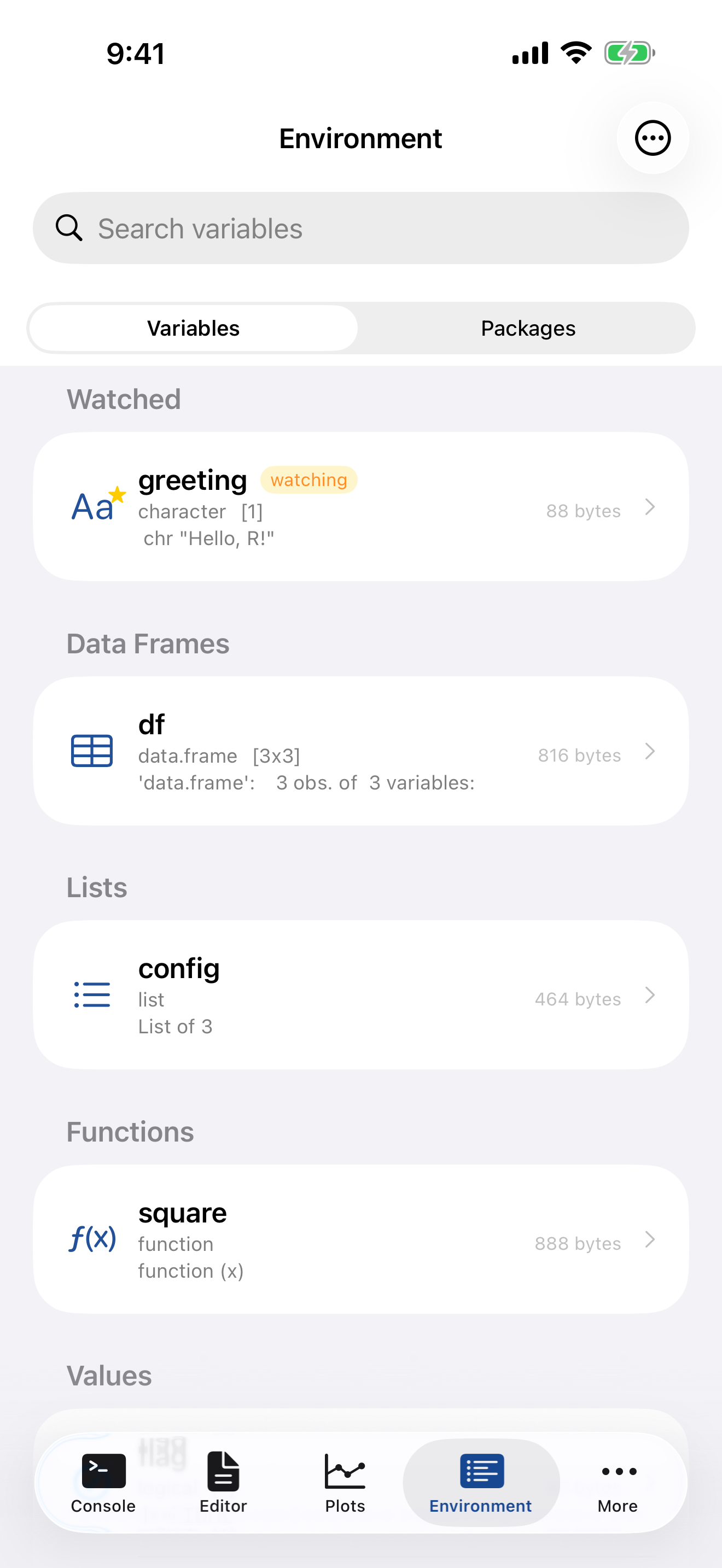
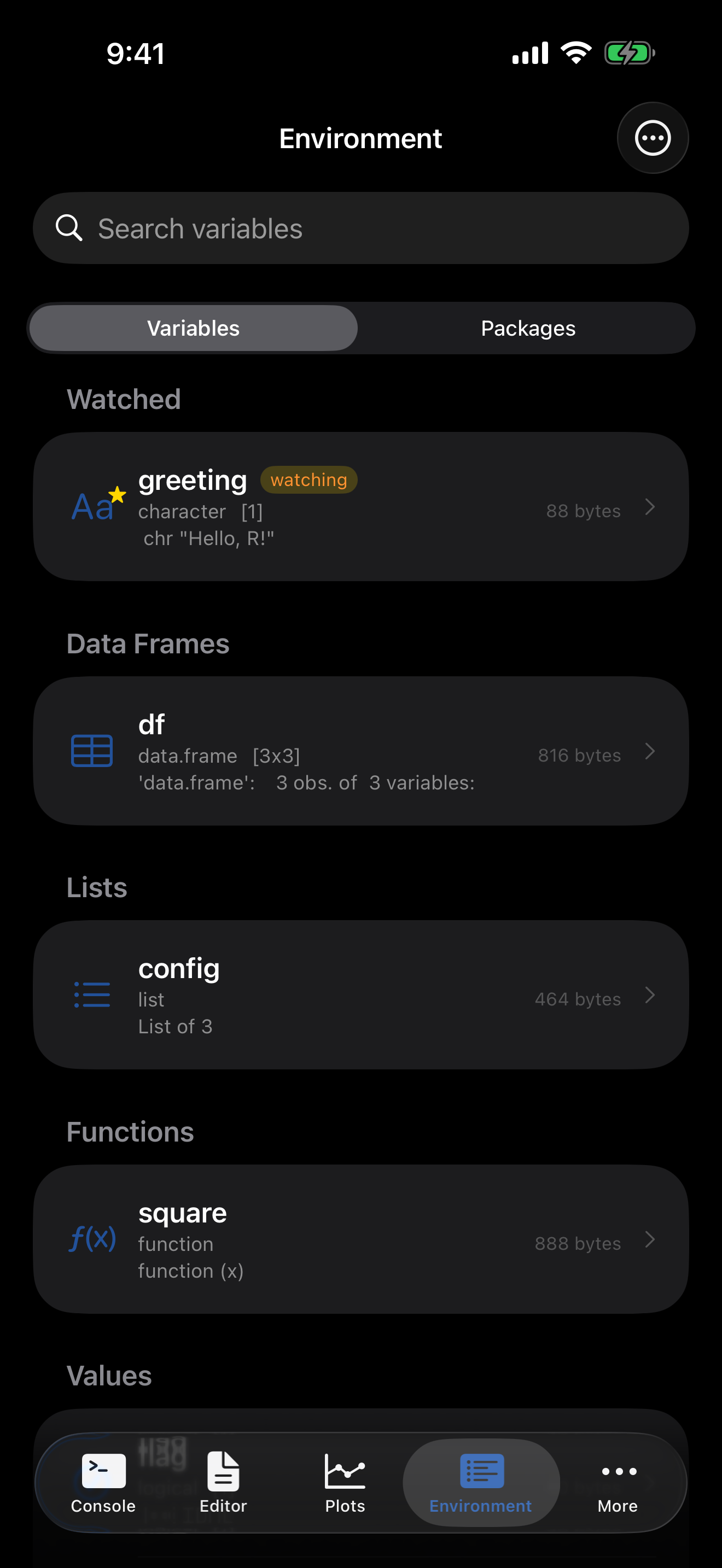
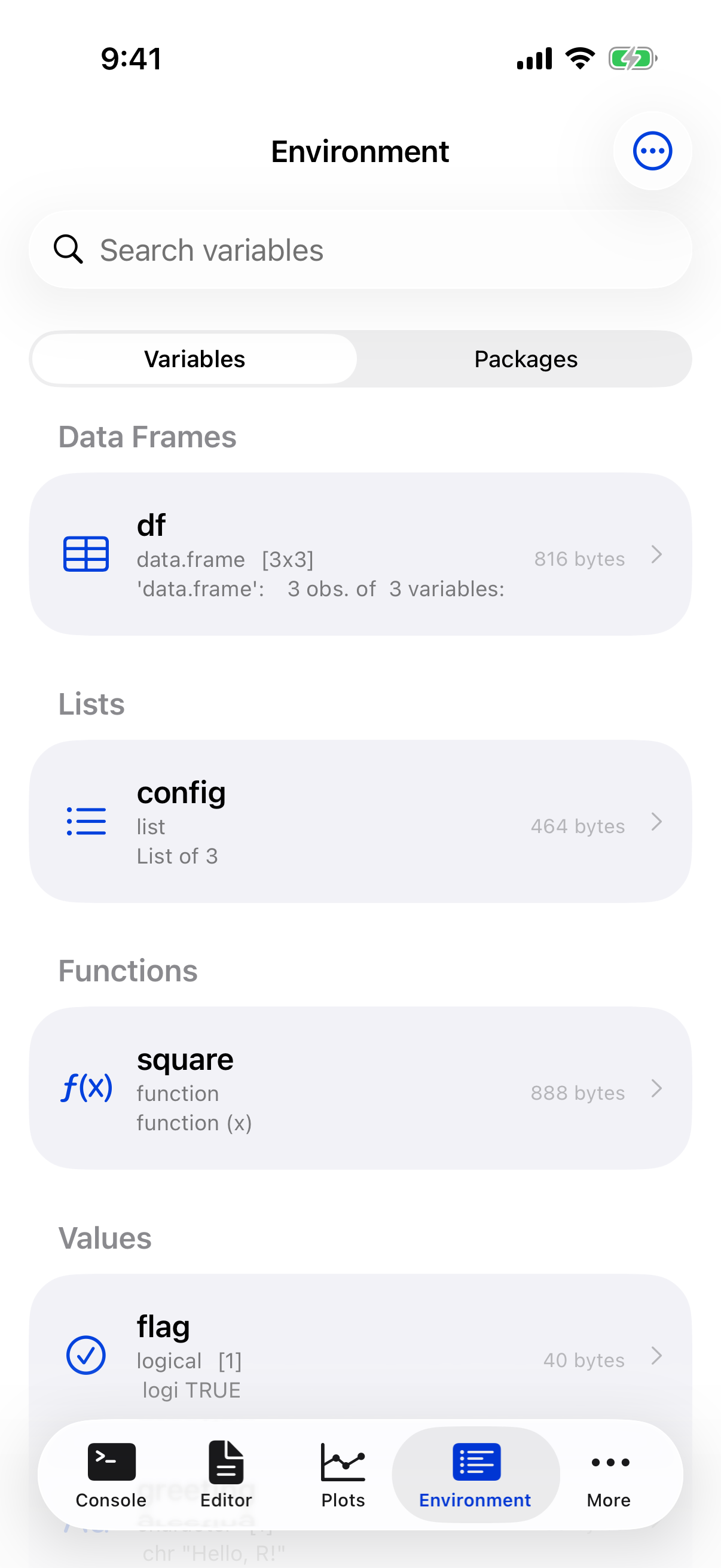
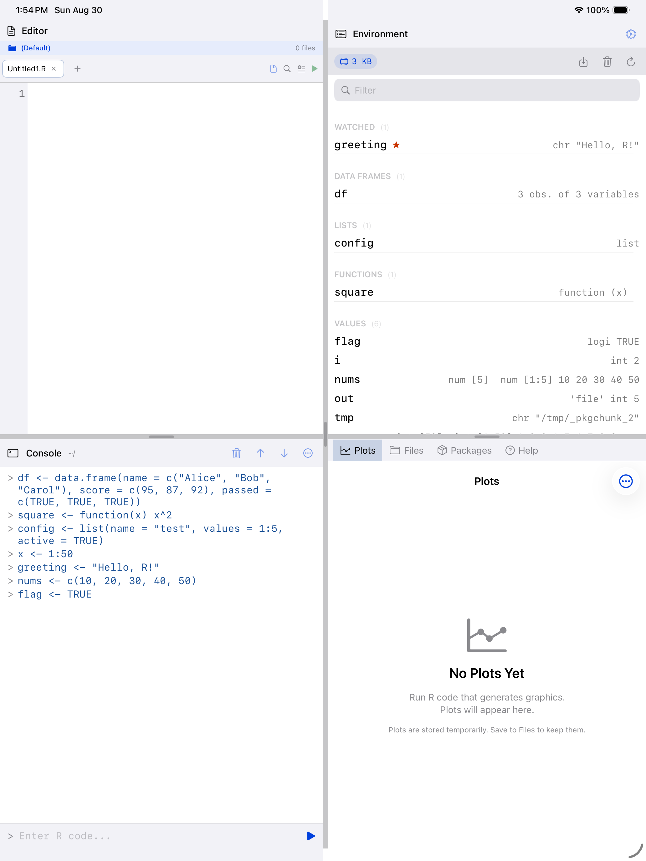
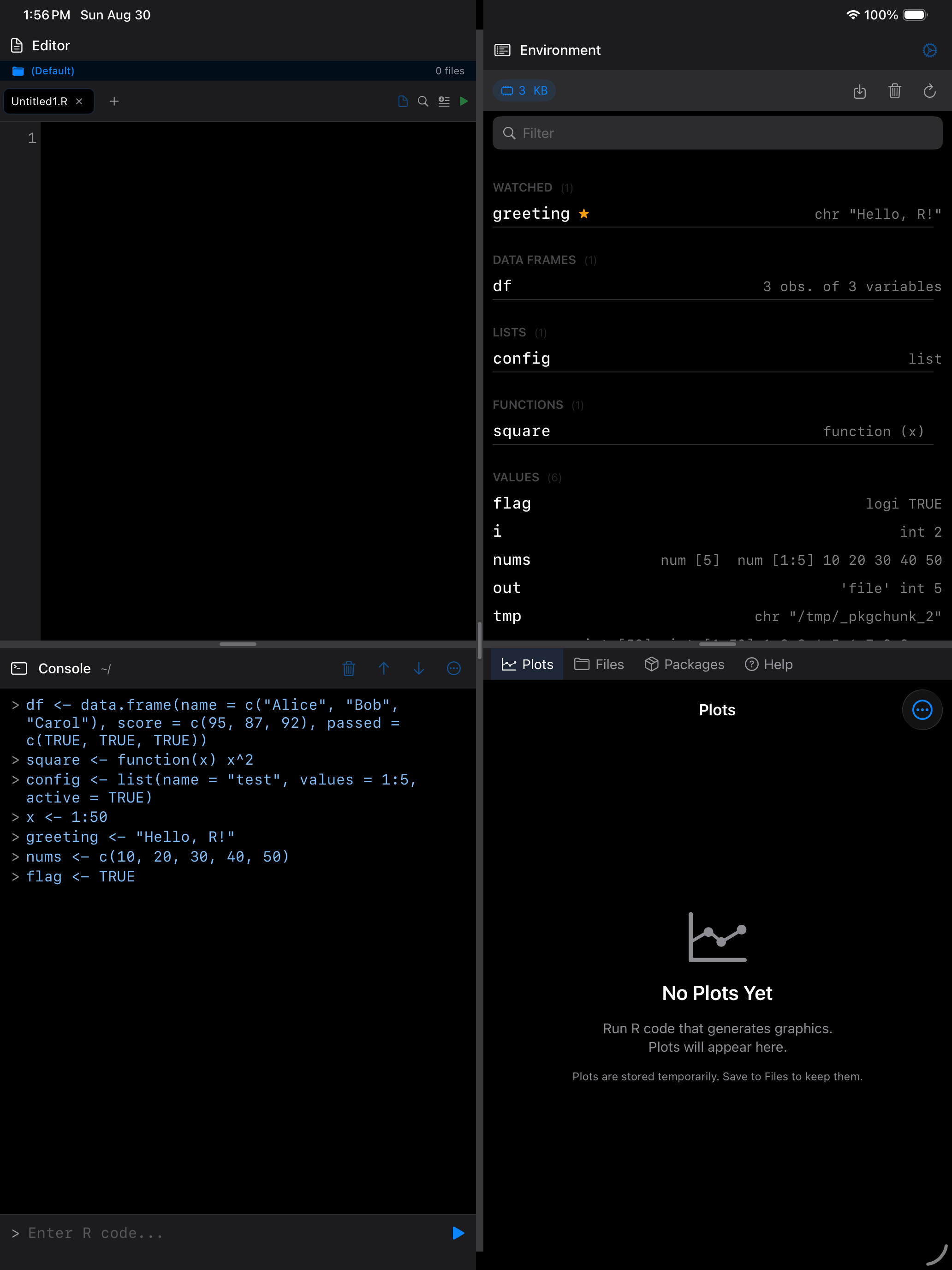
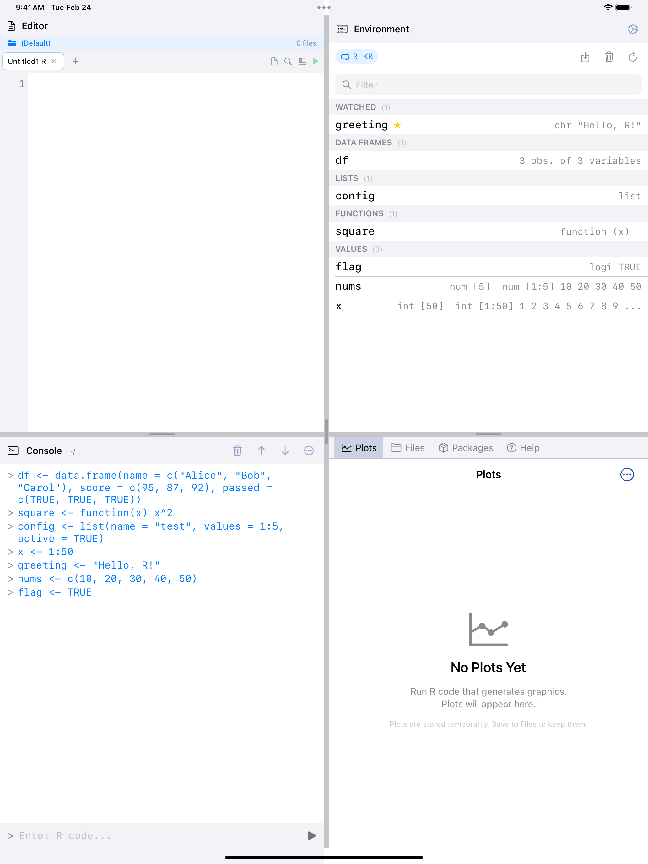
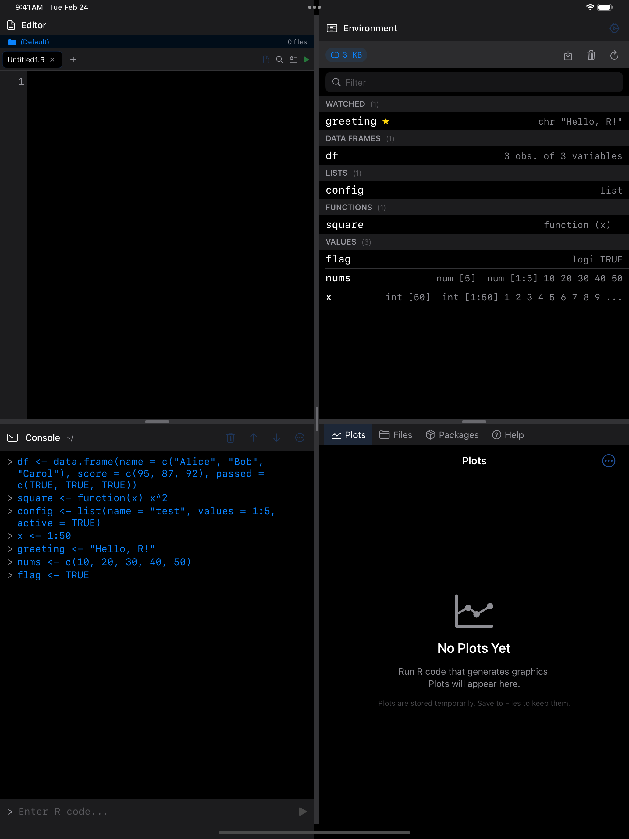
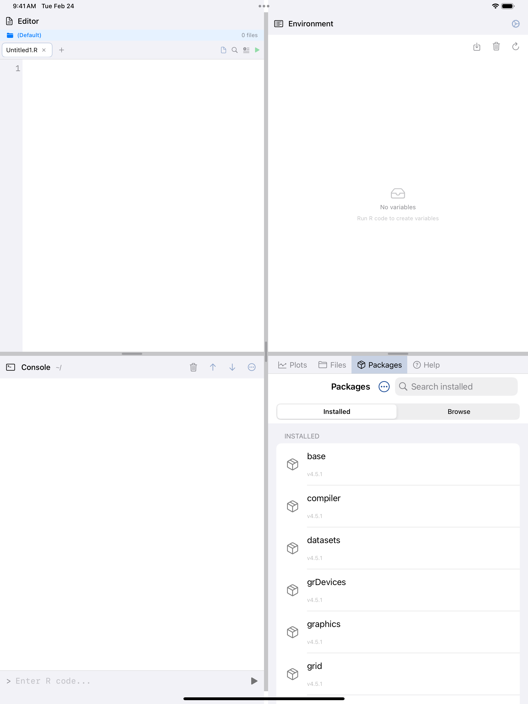
The Environment tab shows every variable in your R session at a glance: names, types, sizes, and value previews, all updated in real time.
Your variables, at a glance
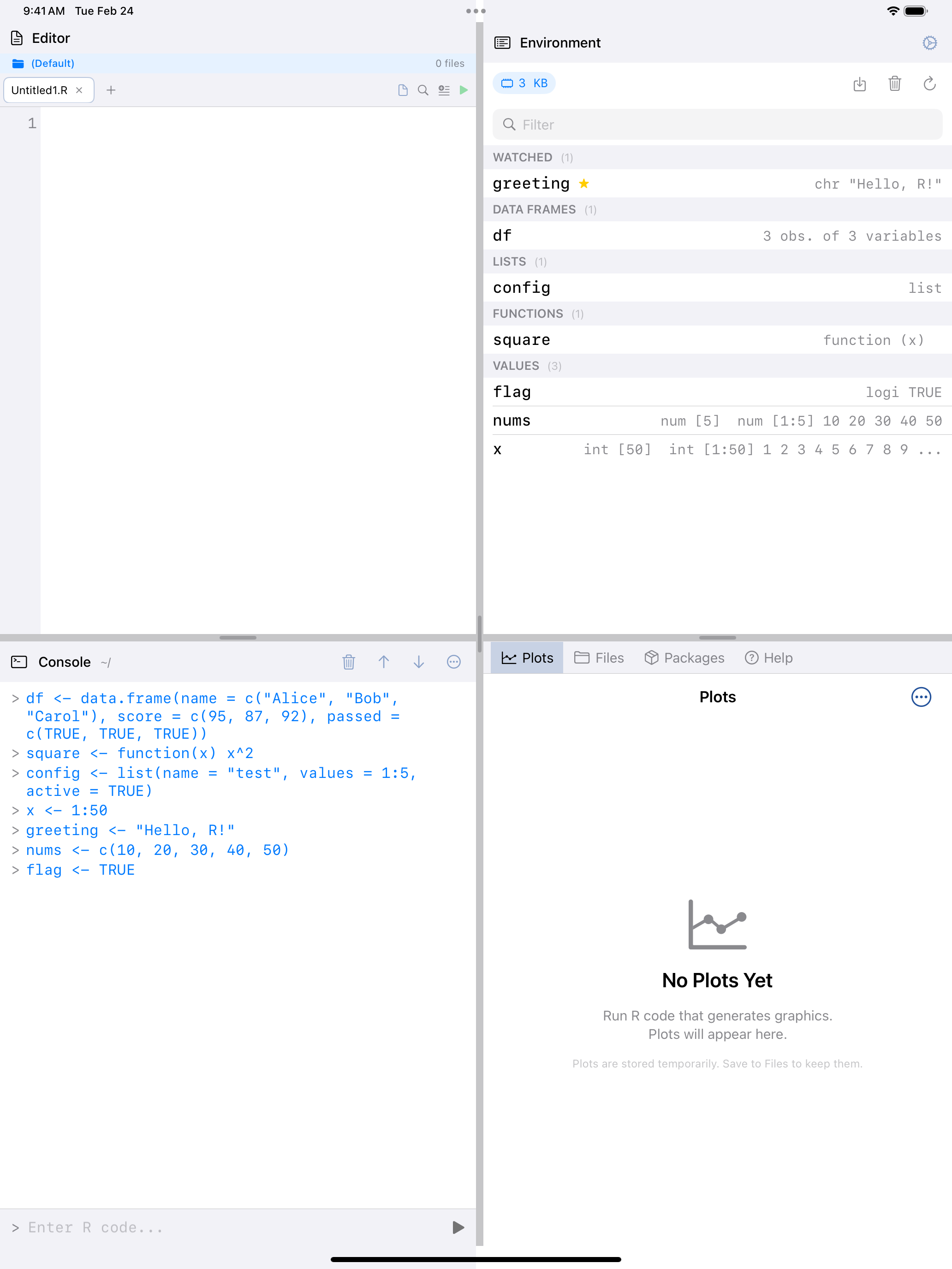
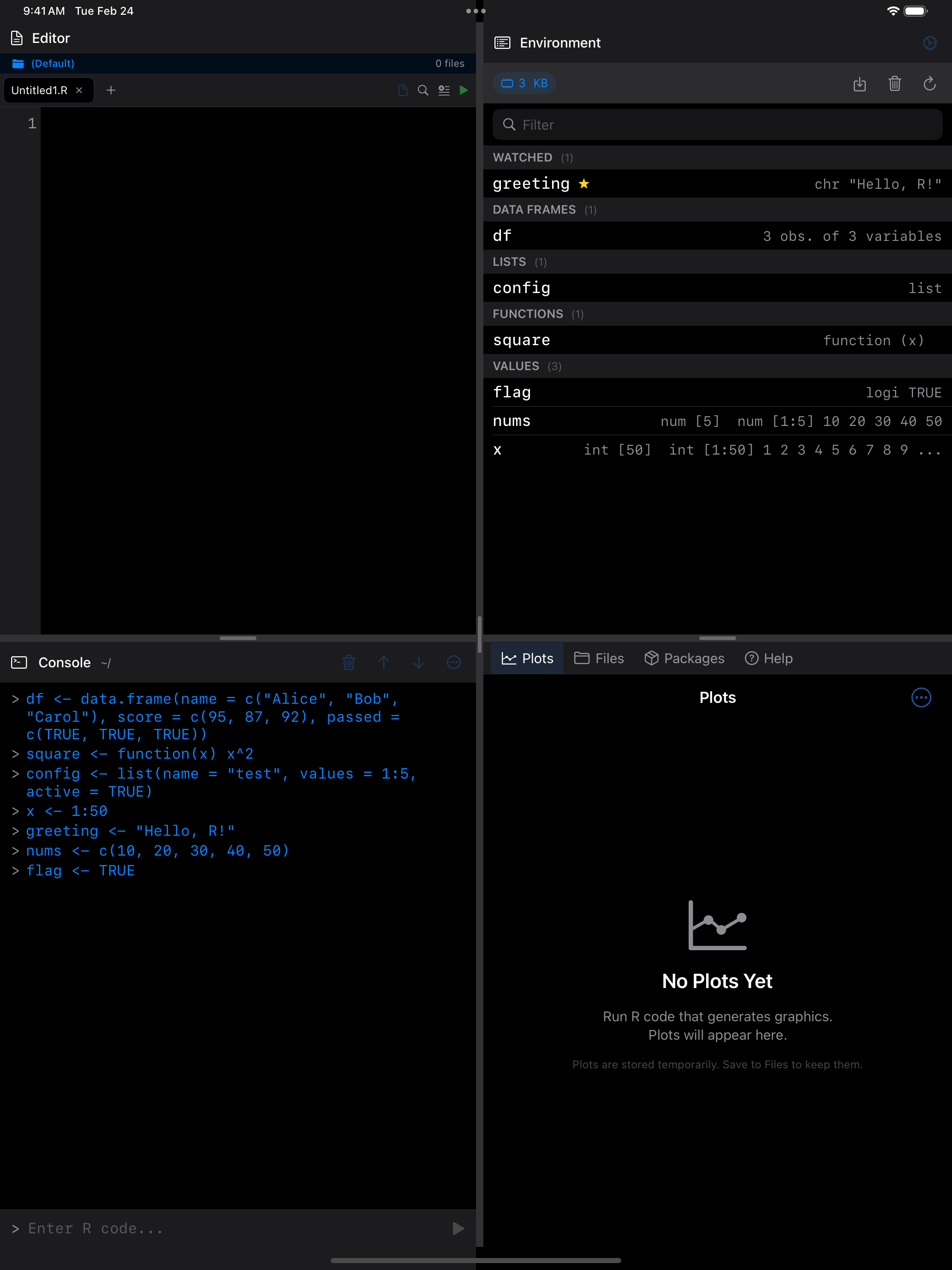
Once you start creating variables in the Console or Editor, they show up here automatically. The list refreshes in real time, so you will see new variables appear right after you create them.
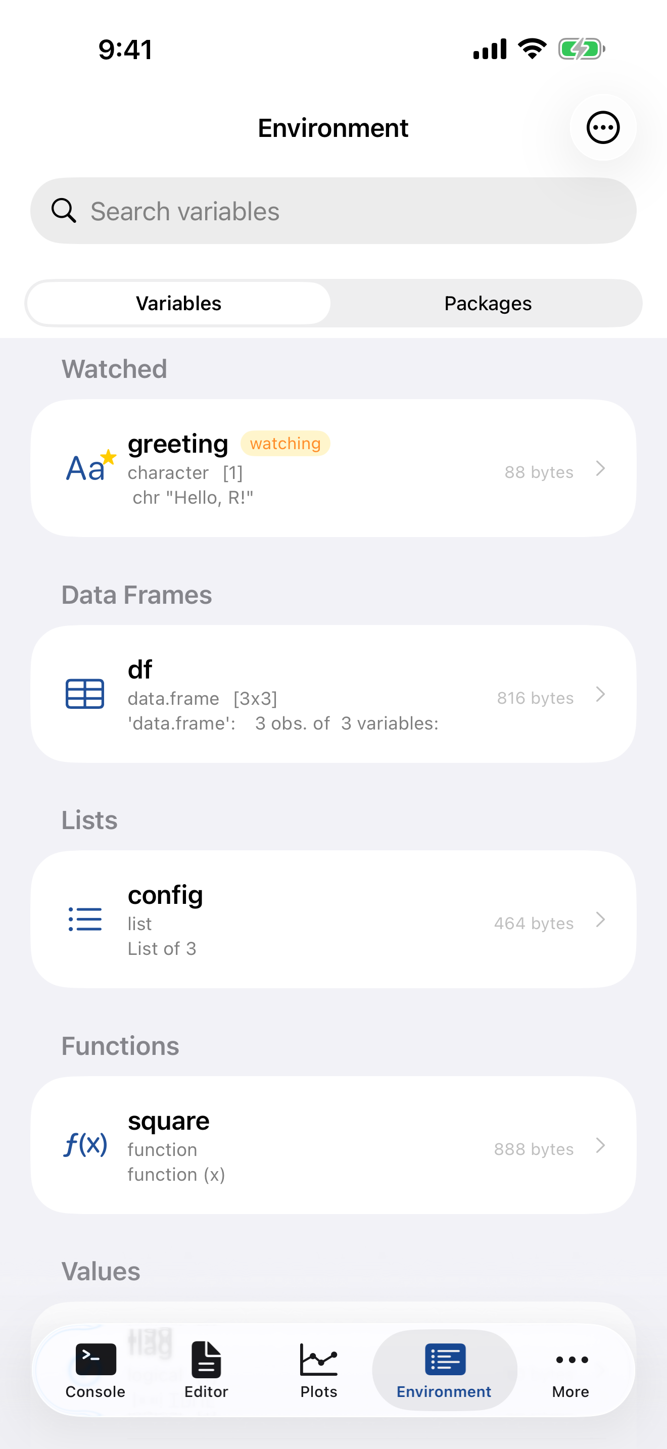
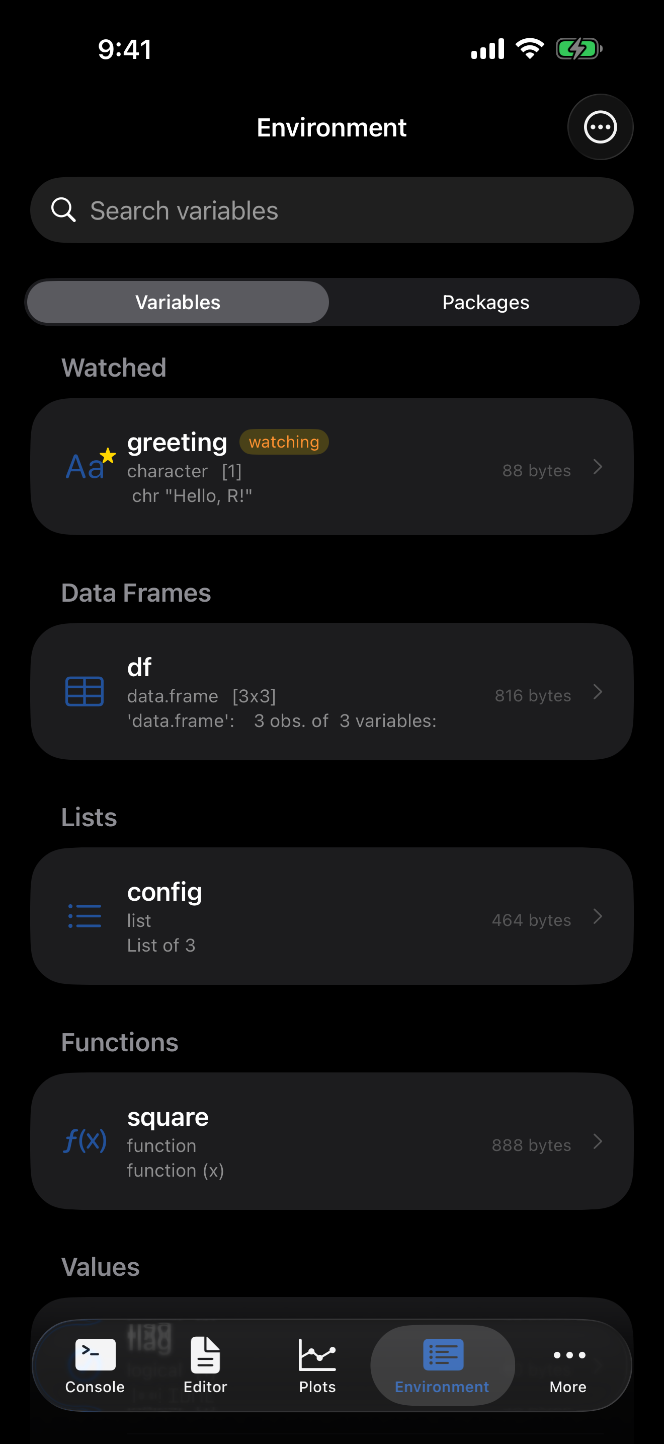
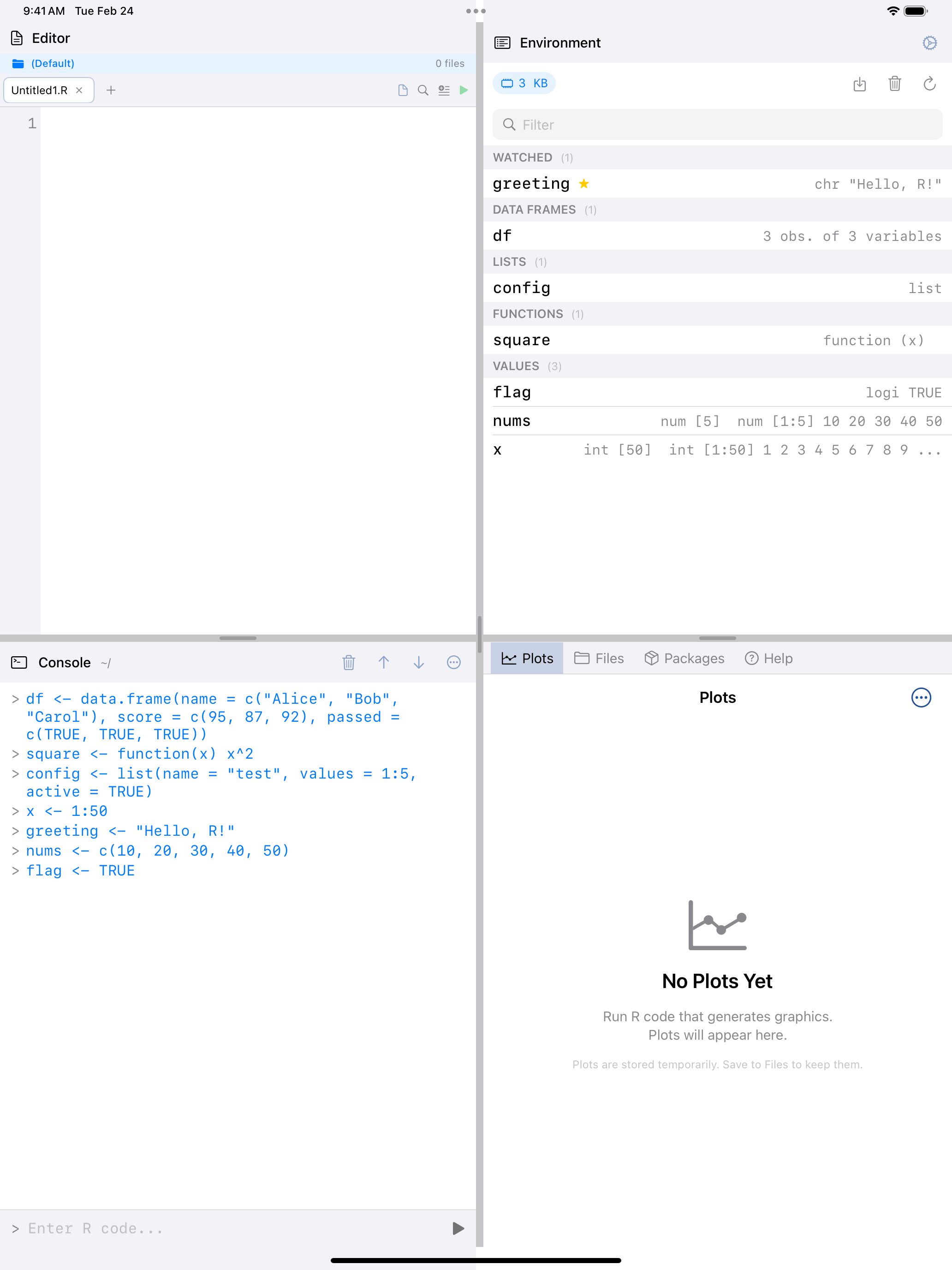
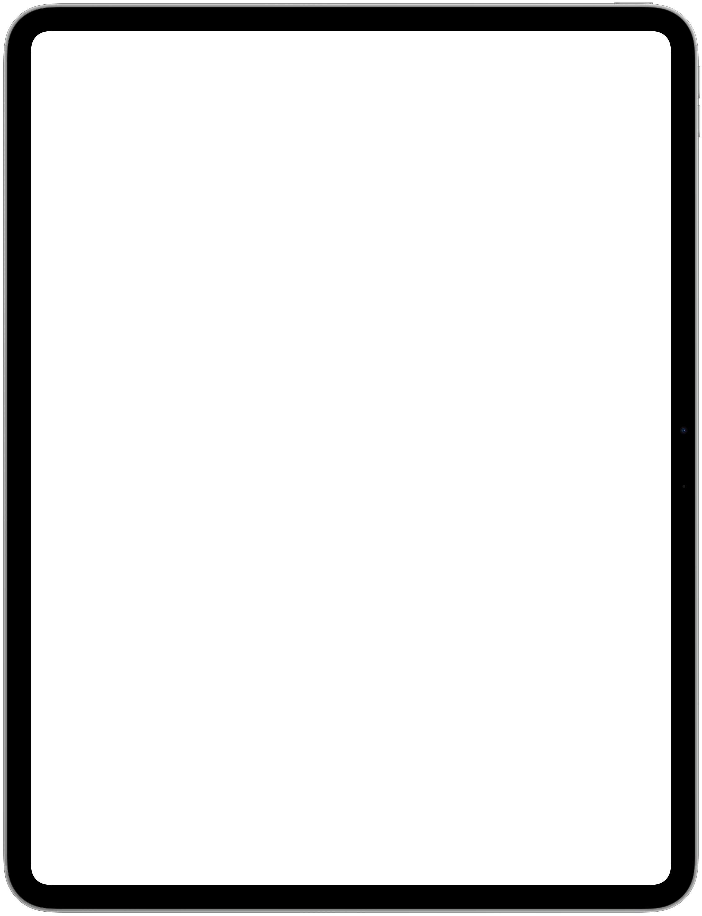
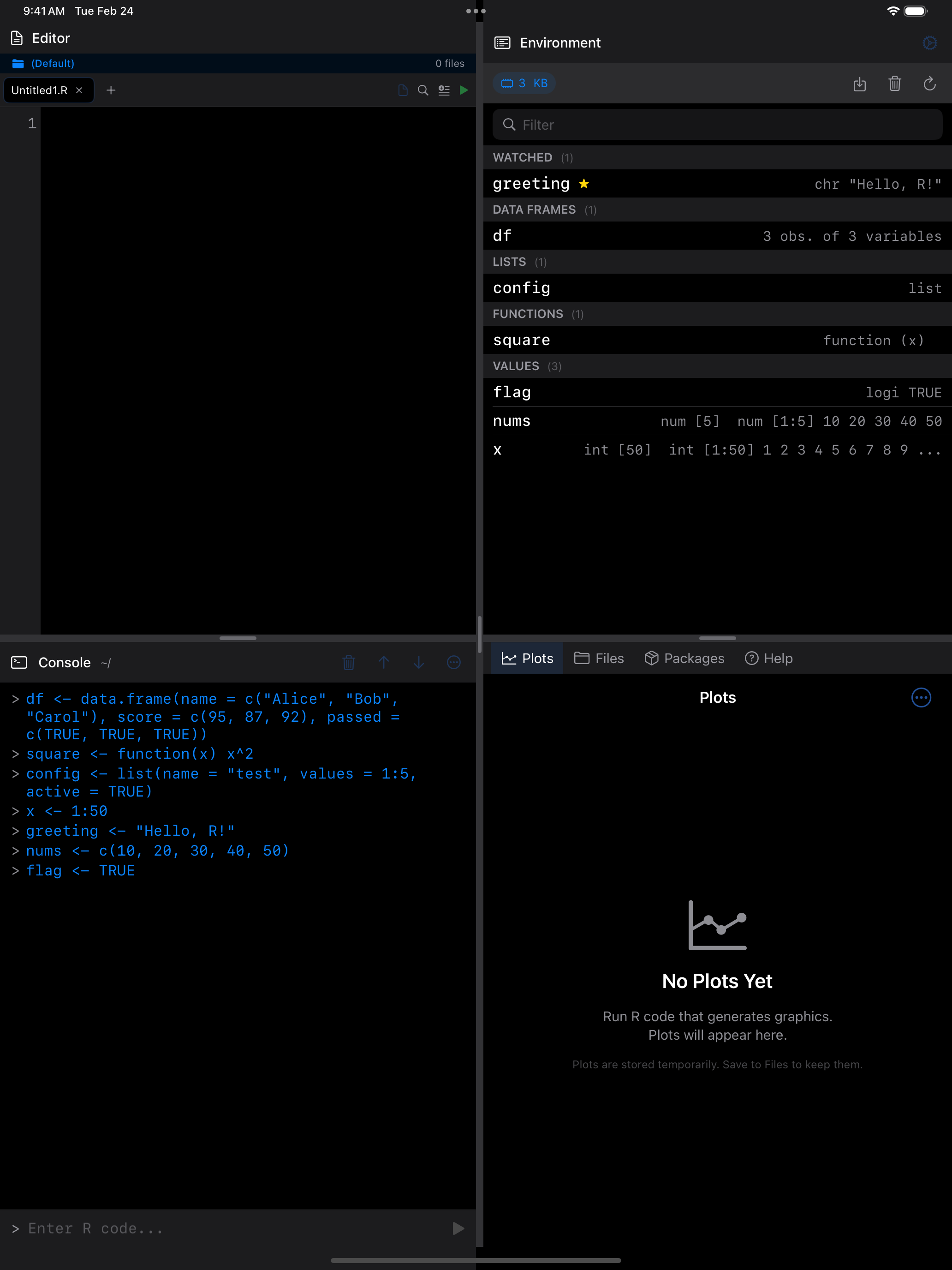
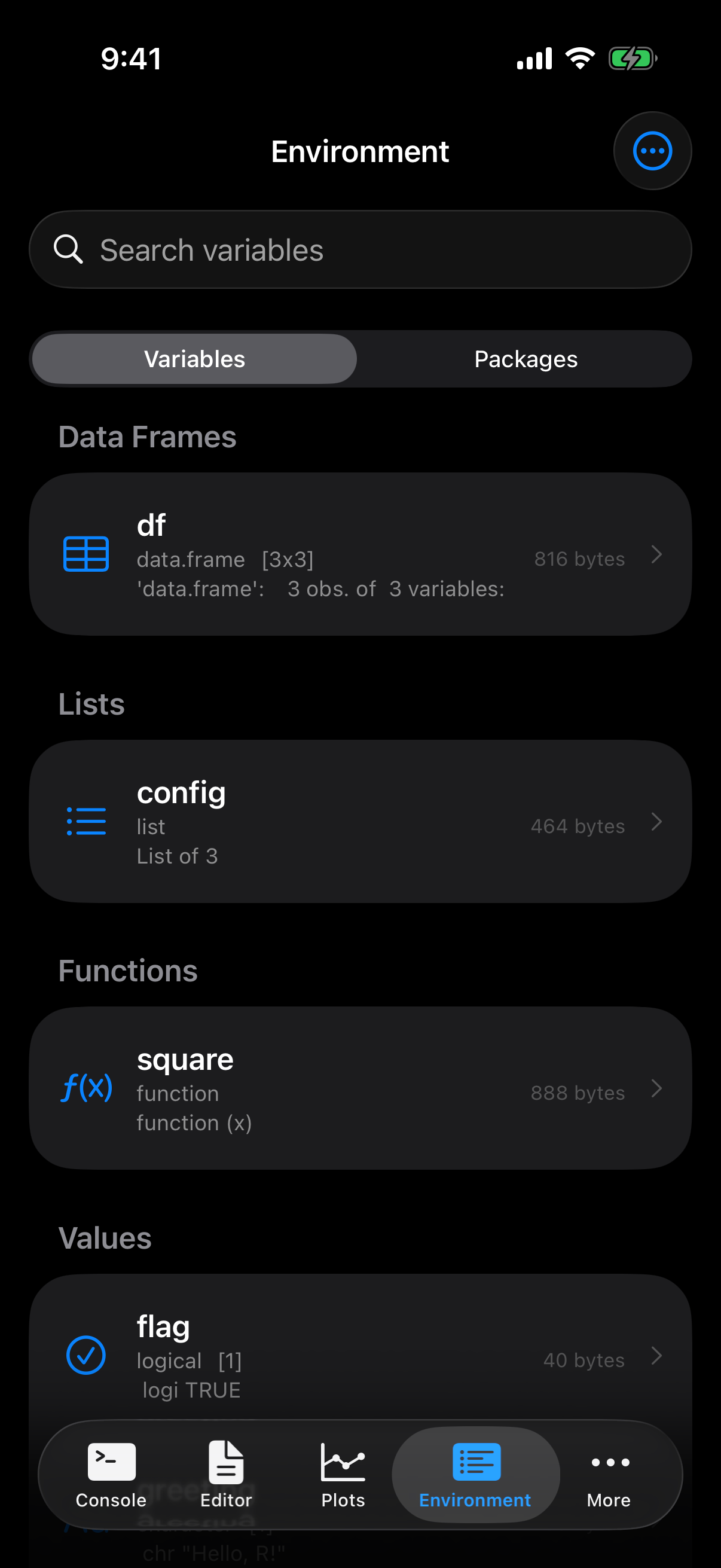
Each row shows the variable’s name, class (like data.frame or numeric), memory size, and a short preview of its contents.
How variables are organized
Variables are grouped by R type:
- Data Frames: includes
data.frame,tibble, anddata.tableobjects - Matrices:
matrixandarraytypes - Lists: nested list structures
- Functions: any custom functions you have defined
- Values: everything else: vectors, scalars, strings, logicals, and so on
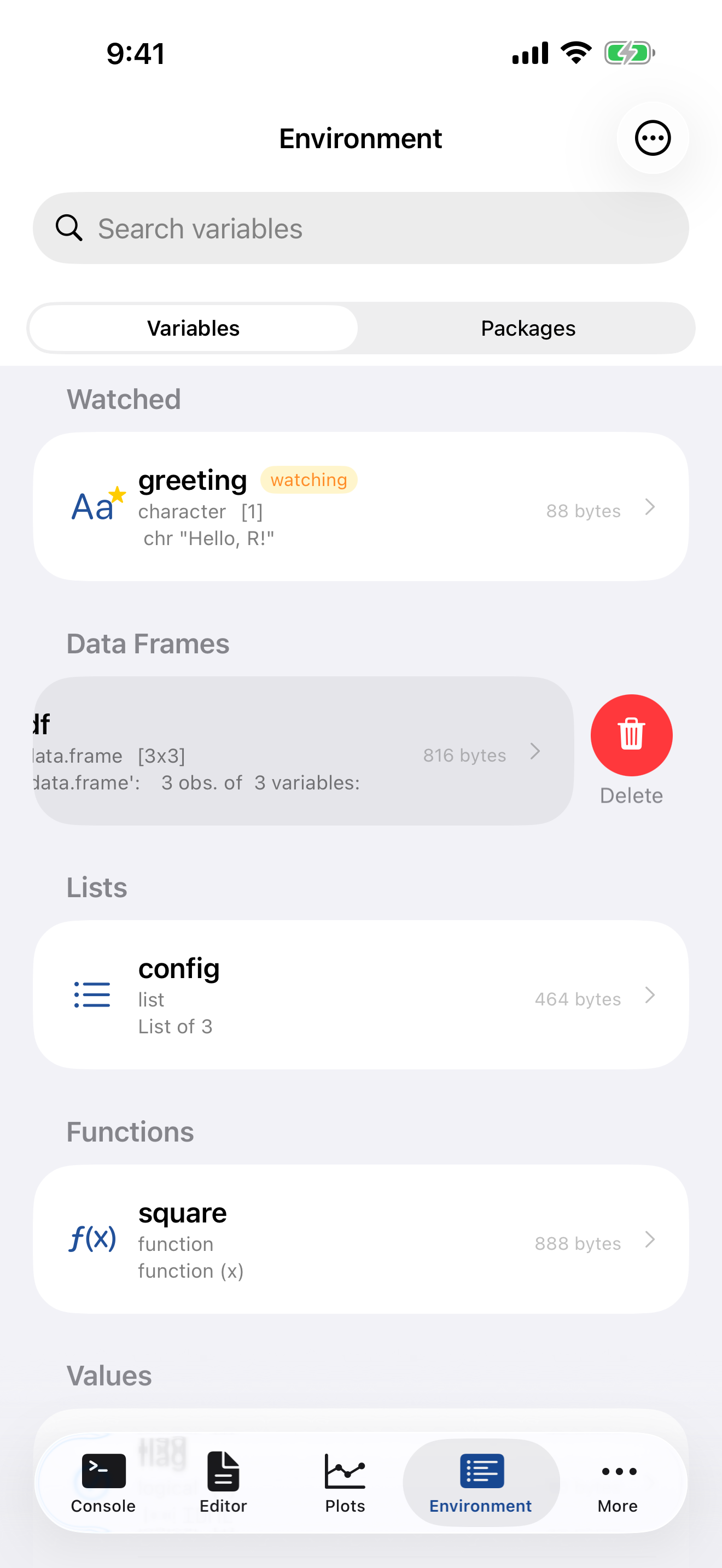
If you have added any variables to your watch list (more on that below), they appear at the very top in their own “Watched” section, regardless of type.
Inspecting a variable in detail
Tap any variable to open a detail sheet. What you see depends on the type.
Data frames show all columns with types and sample values, a preview of the first 10 rows, and an “Open in Data Frame Viewer” button for a full scrollable table.
Vectors and scalars show the full value (up to 15 digits of precision), or a summary and the first 20 elements for longer vectors.
Lists show the str() output and a preview of each element.
Functions show the signature and body.
Other objects, such as a model from lm(), a formula or an environment, are described with str() in a scrolling block.
Every detail view includes a Copy as R Code section; tap View Code for the dput() output, so you can recreate the variable from scratch or share it. The code is produced when you open it. For objects over 512 KB it isn’t, and the sheet suggests running dput() in the Console instead.
Variables with unusual names, such as `sales 2024`, work everywhere in the Environment; the code it shows you quotes them with backticks.
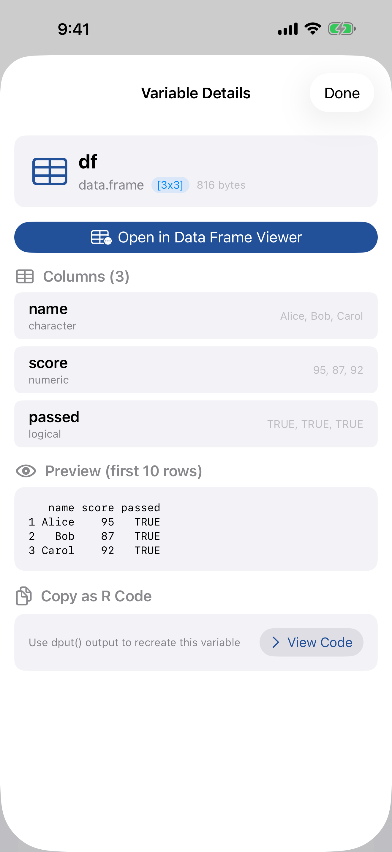
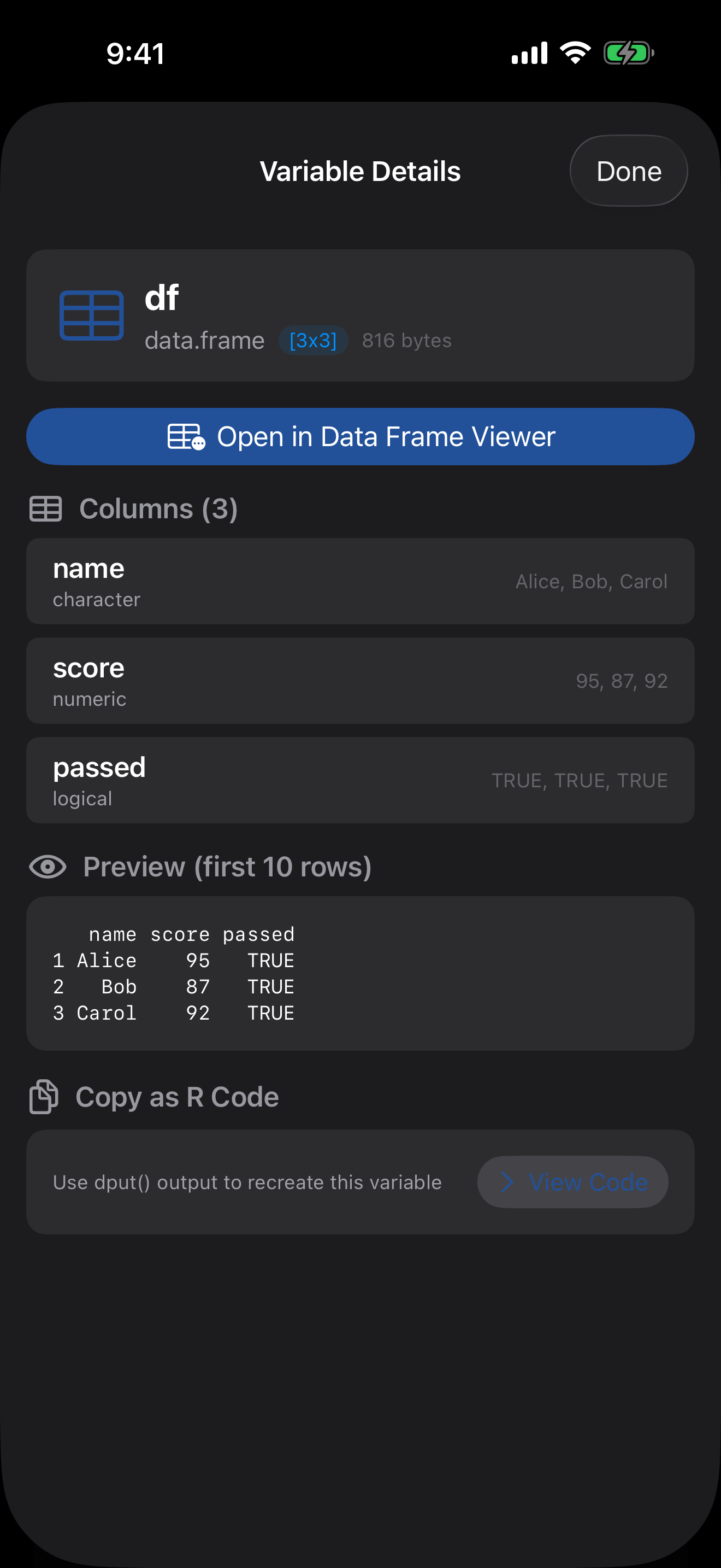
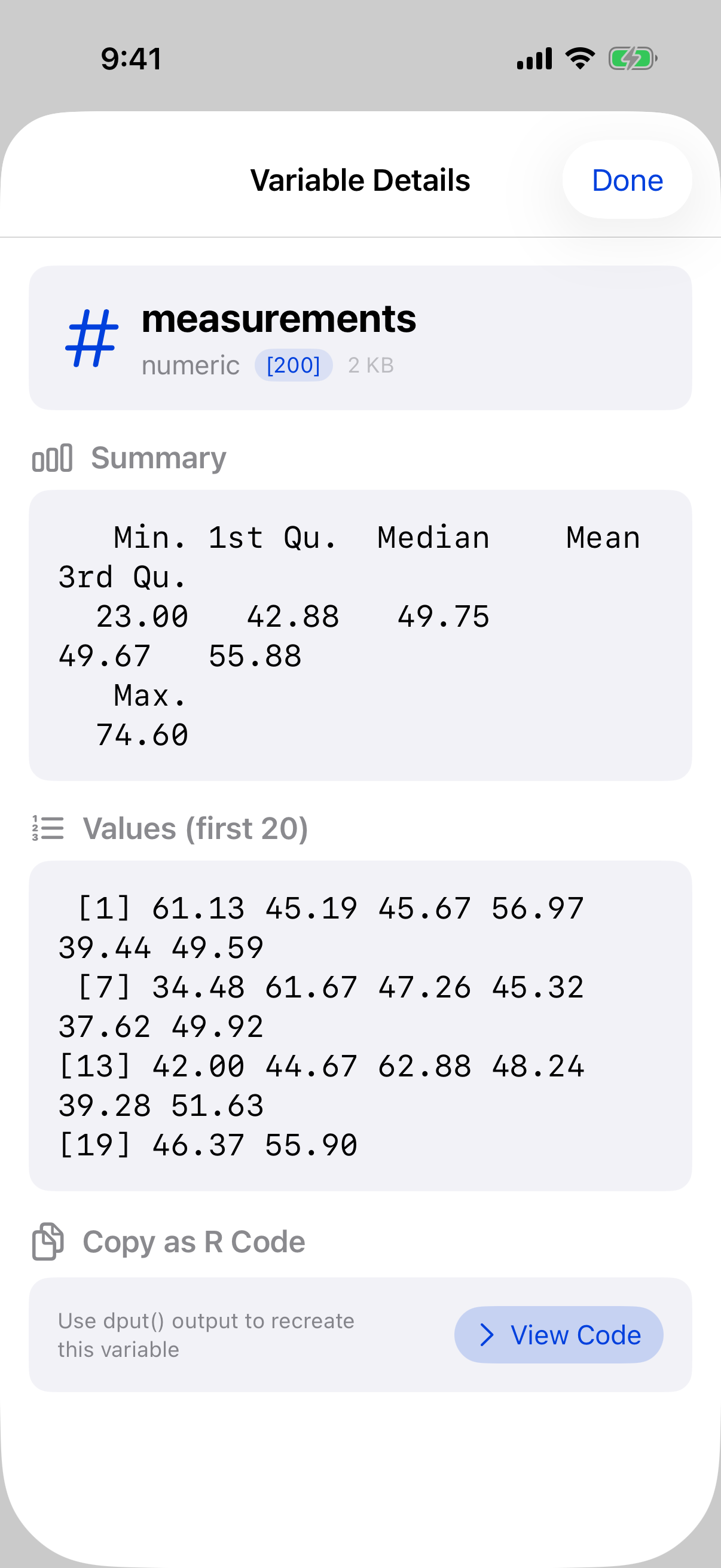
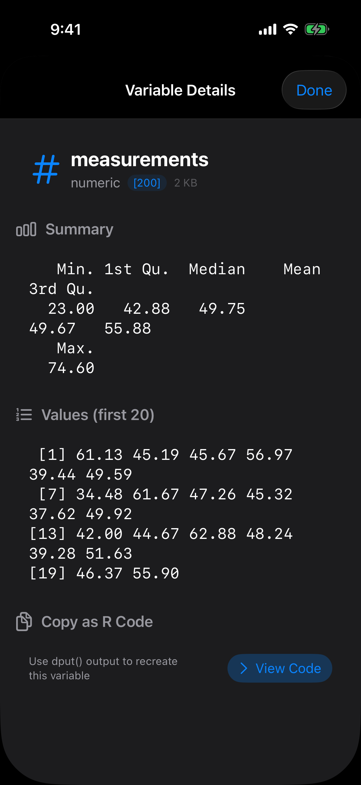
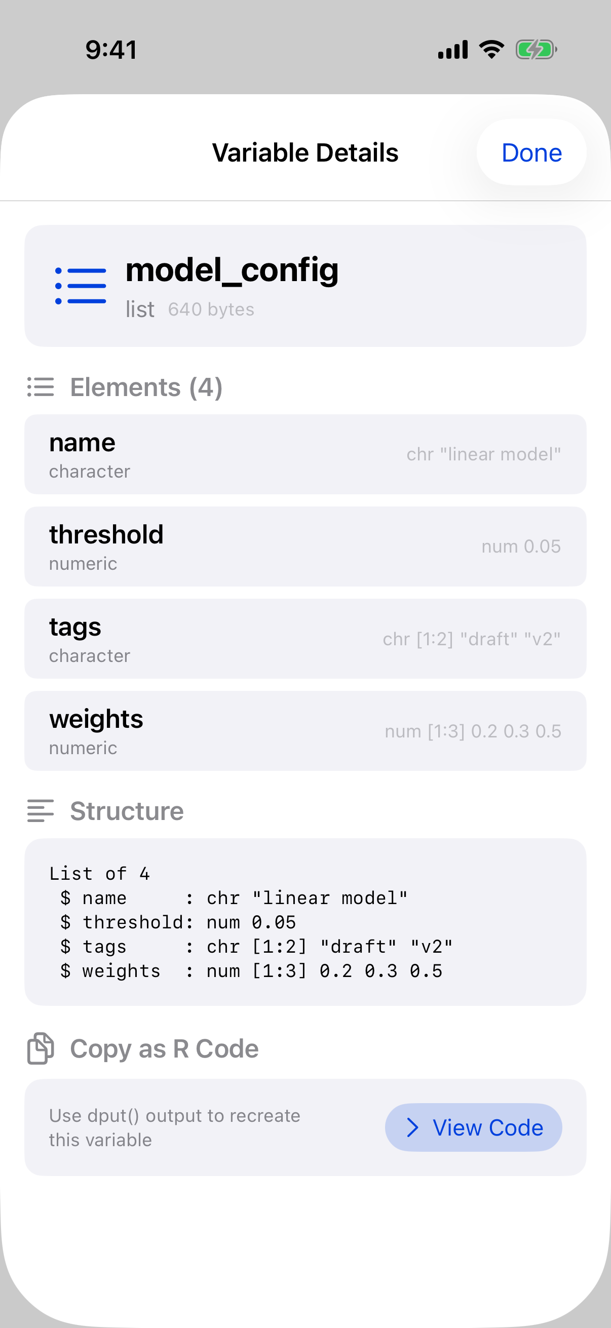
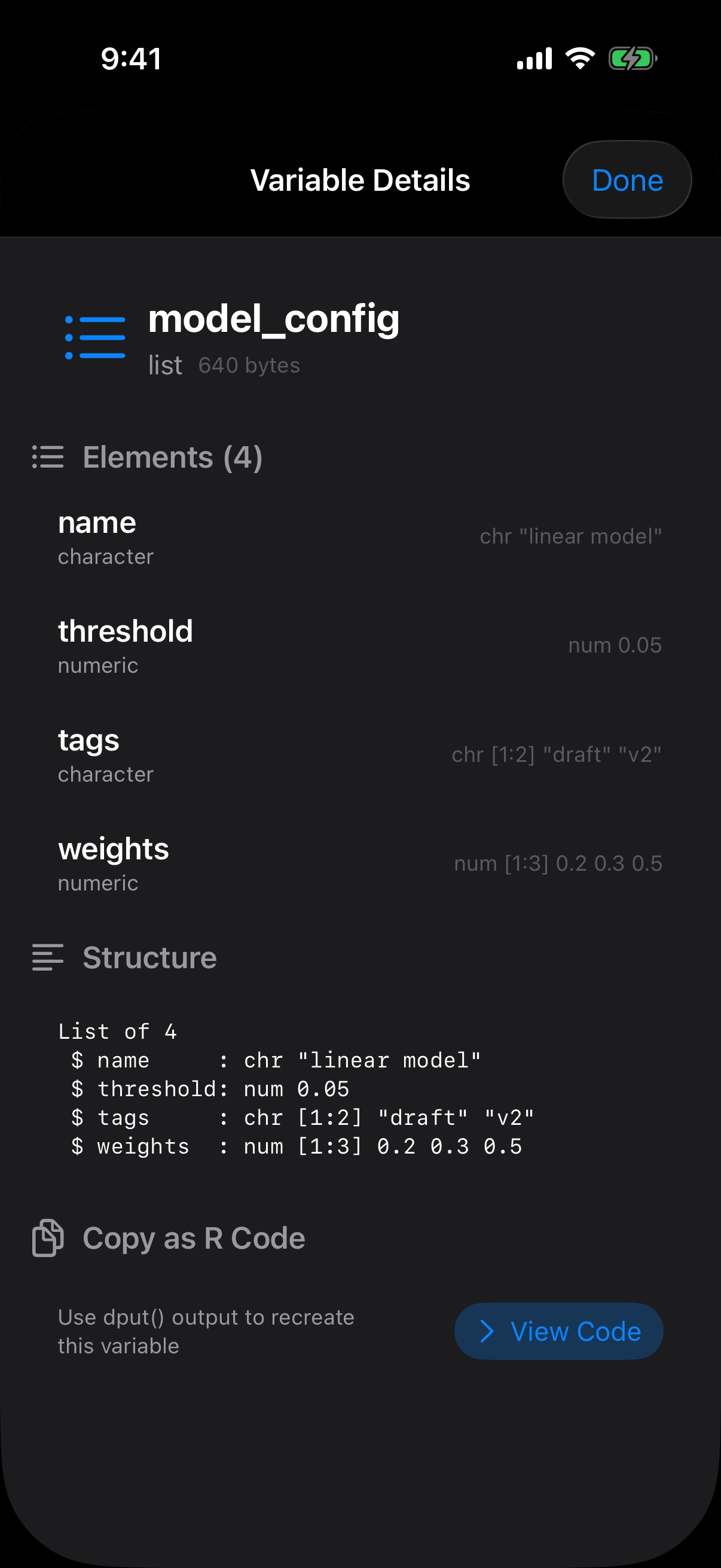
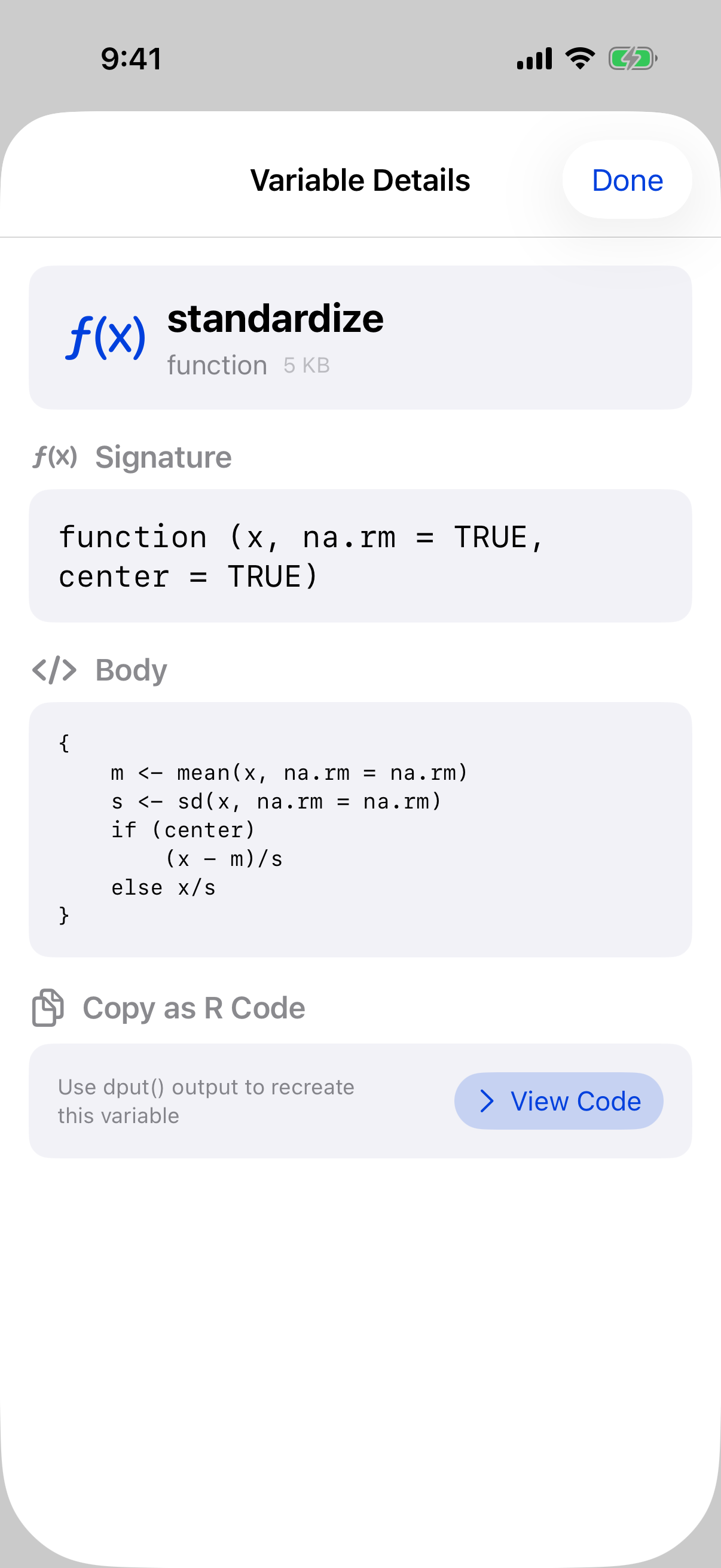
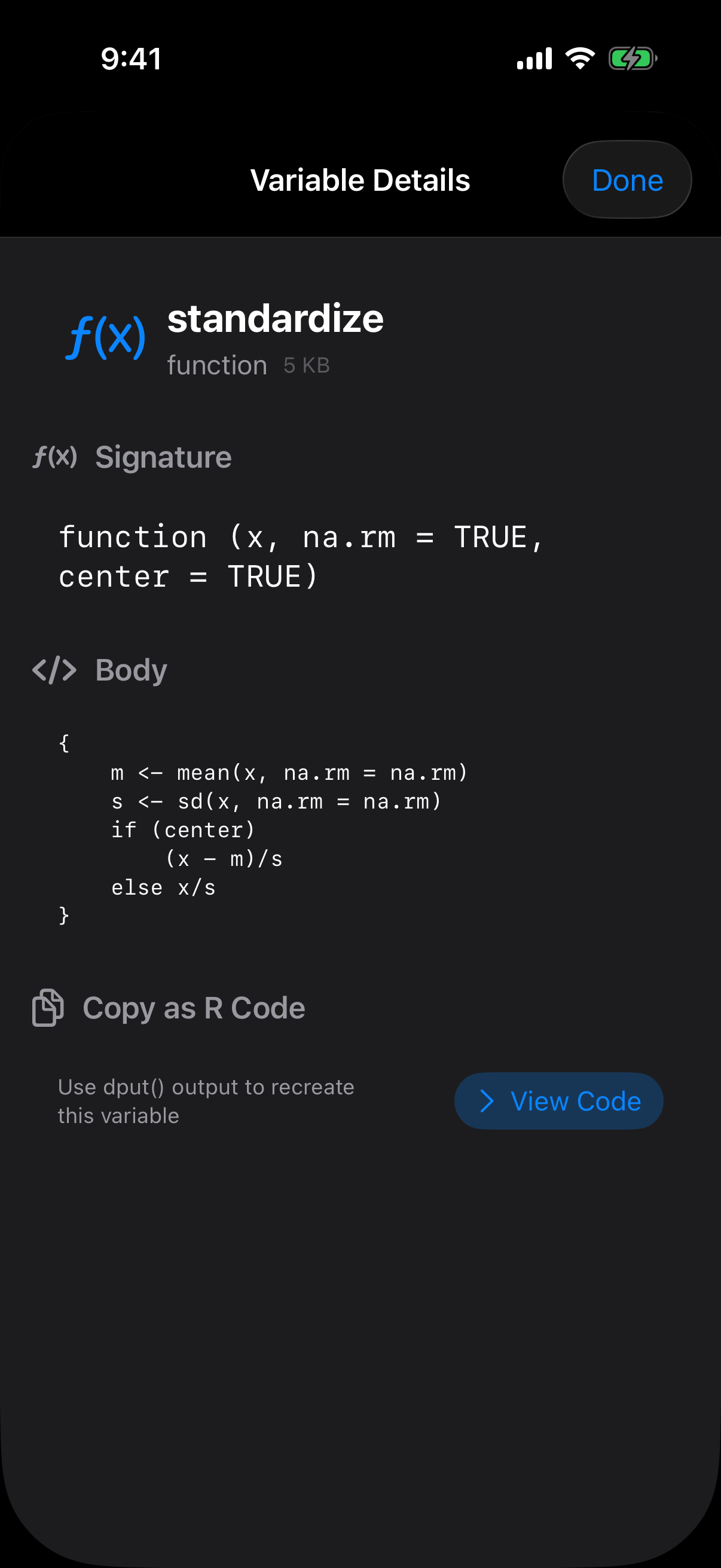
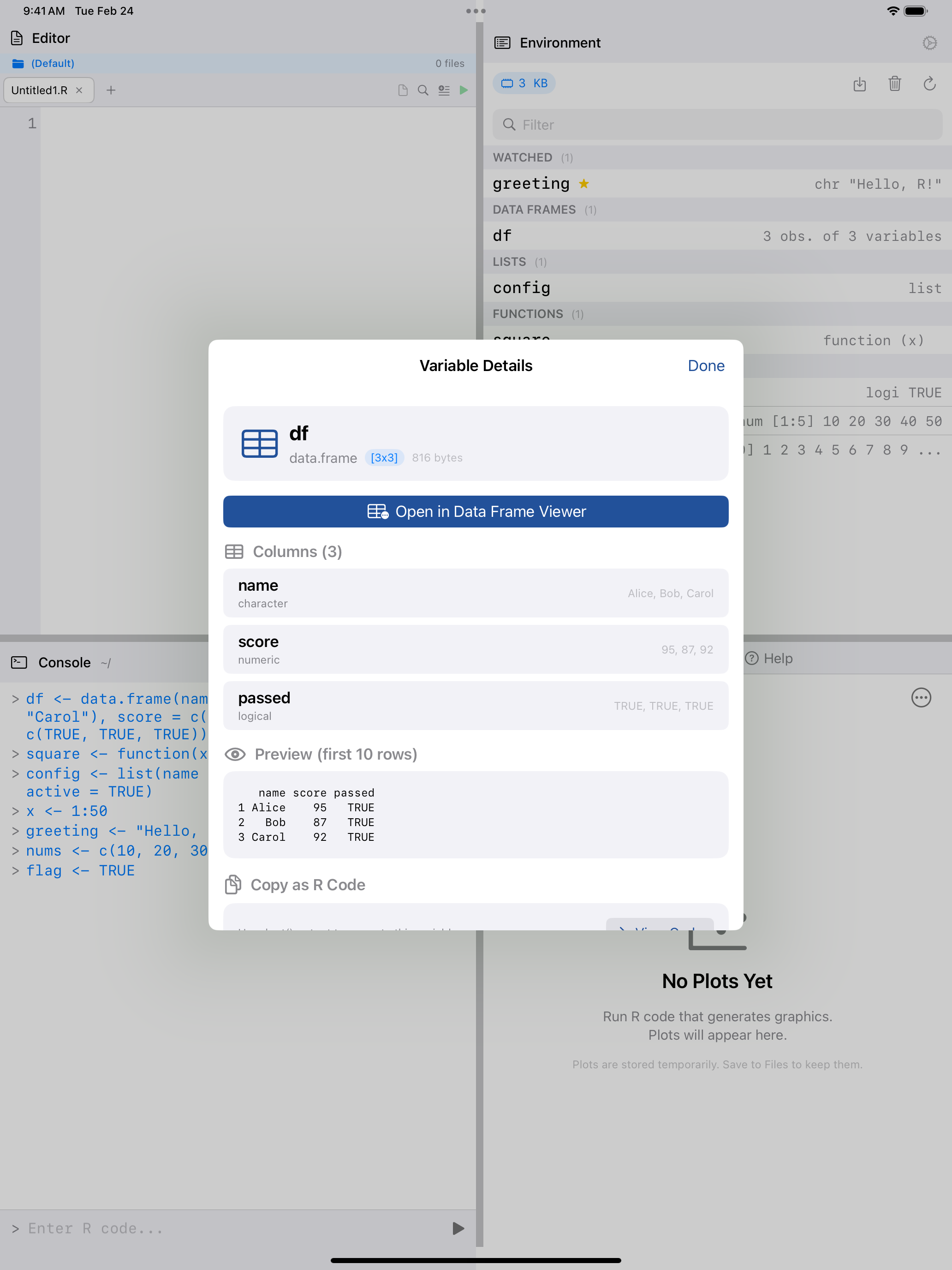
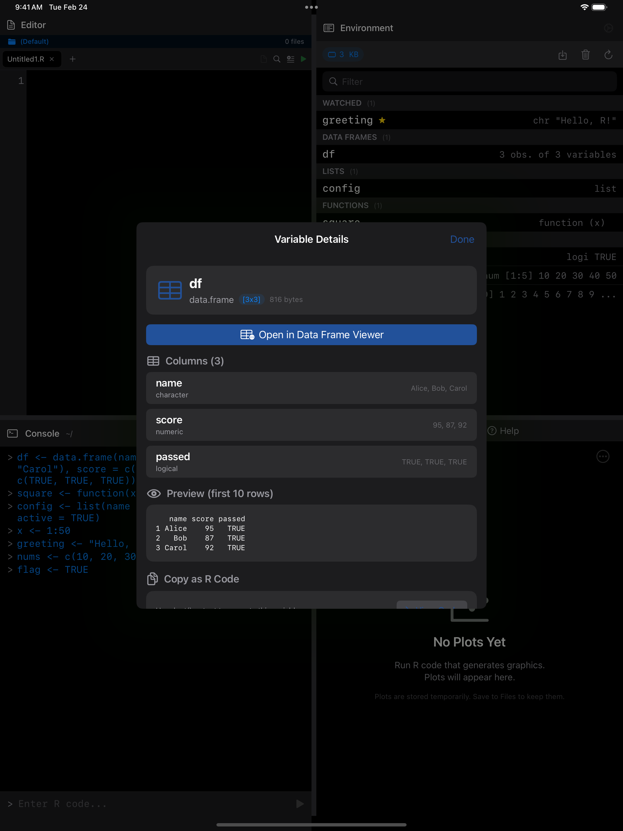
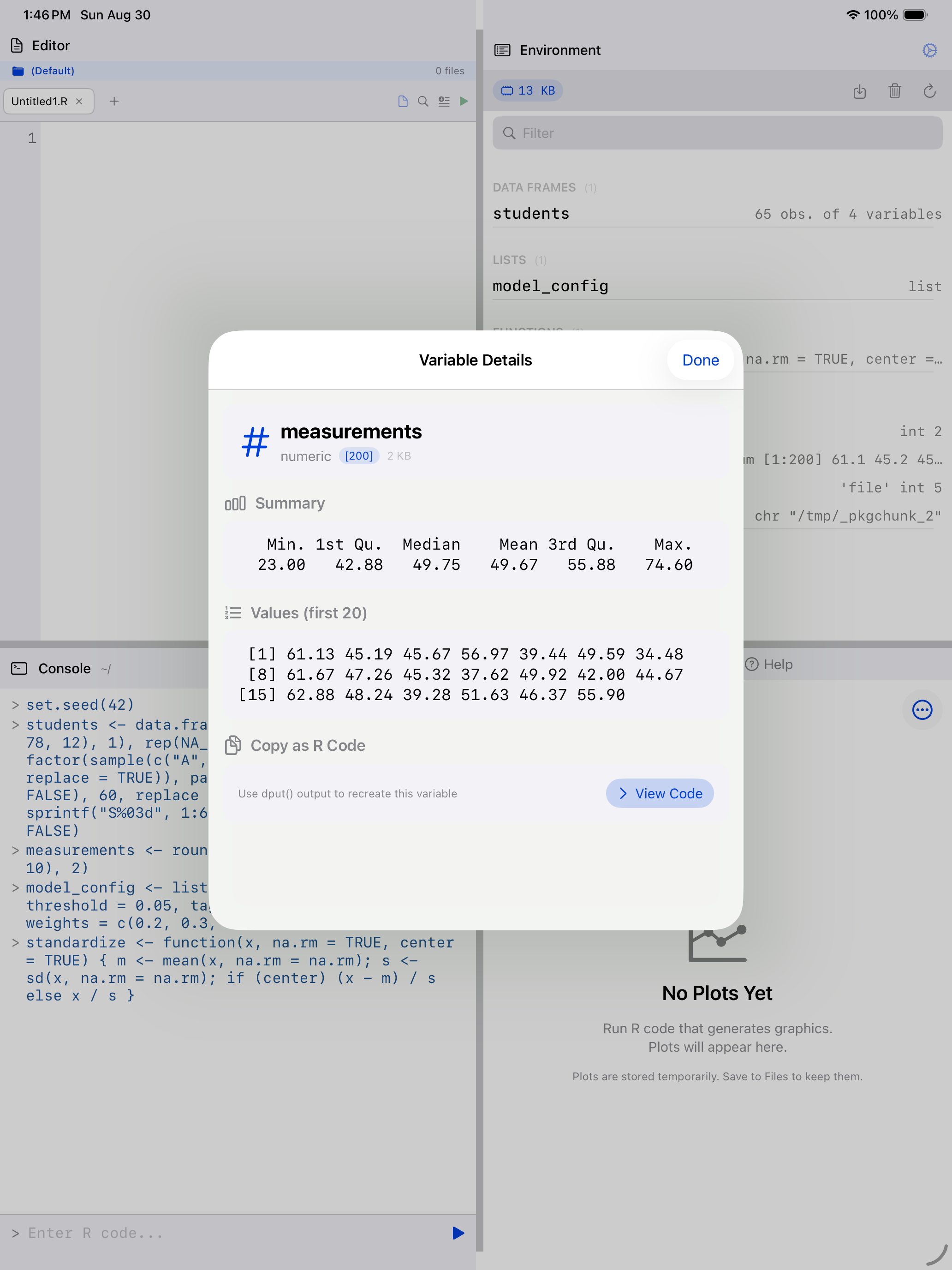
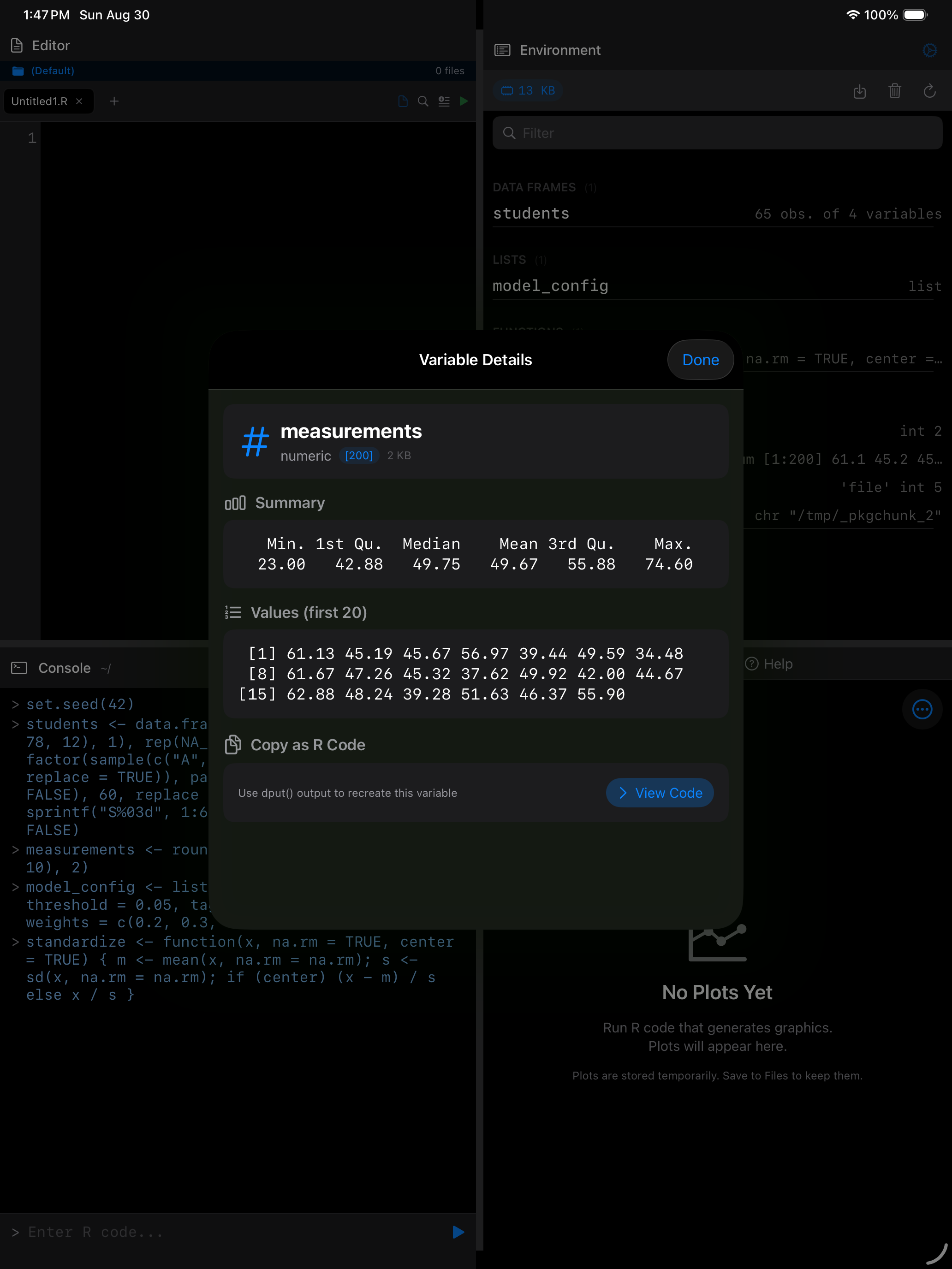
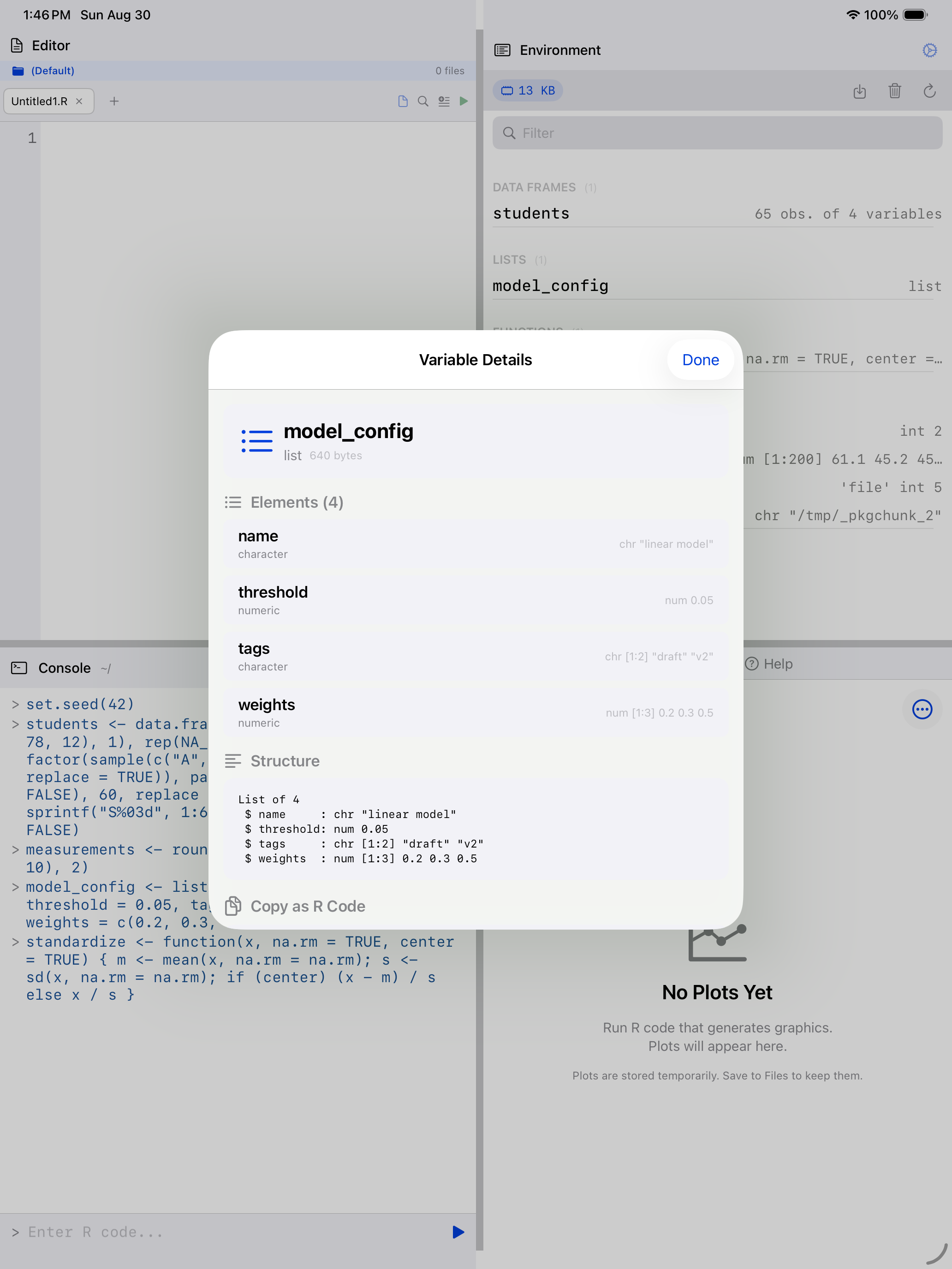
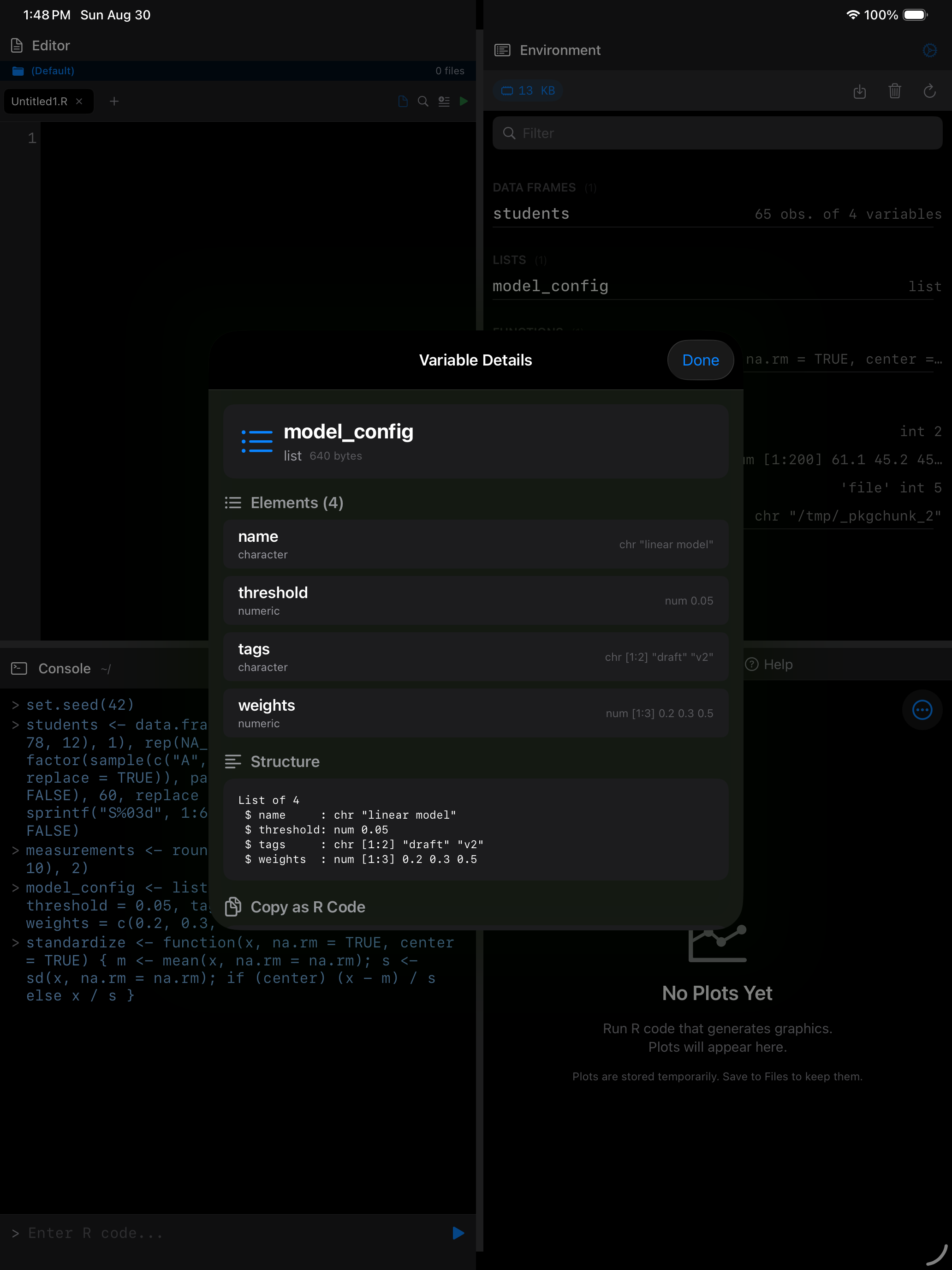
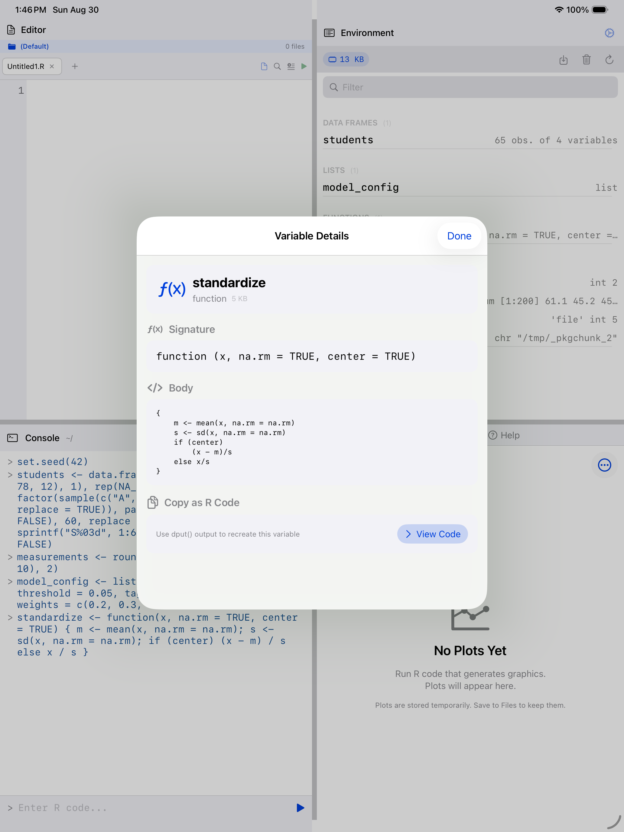
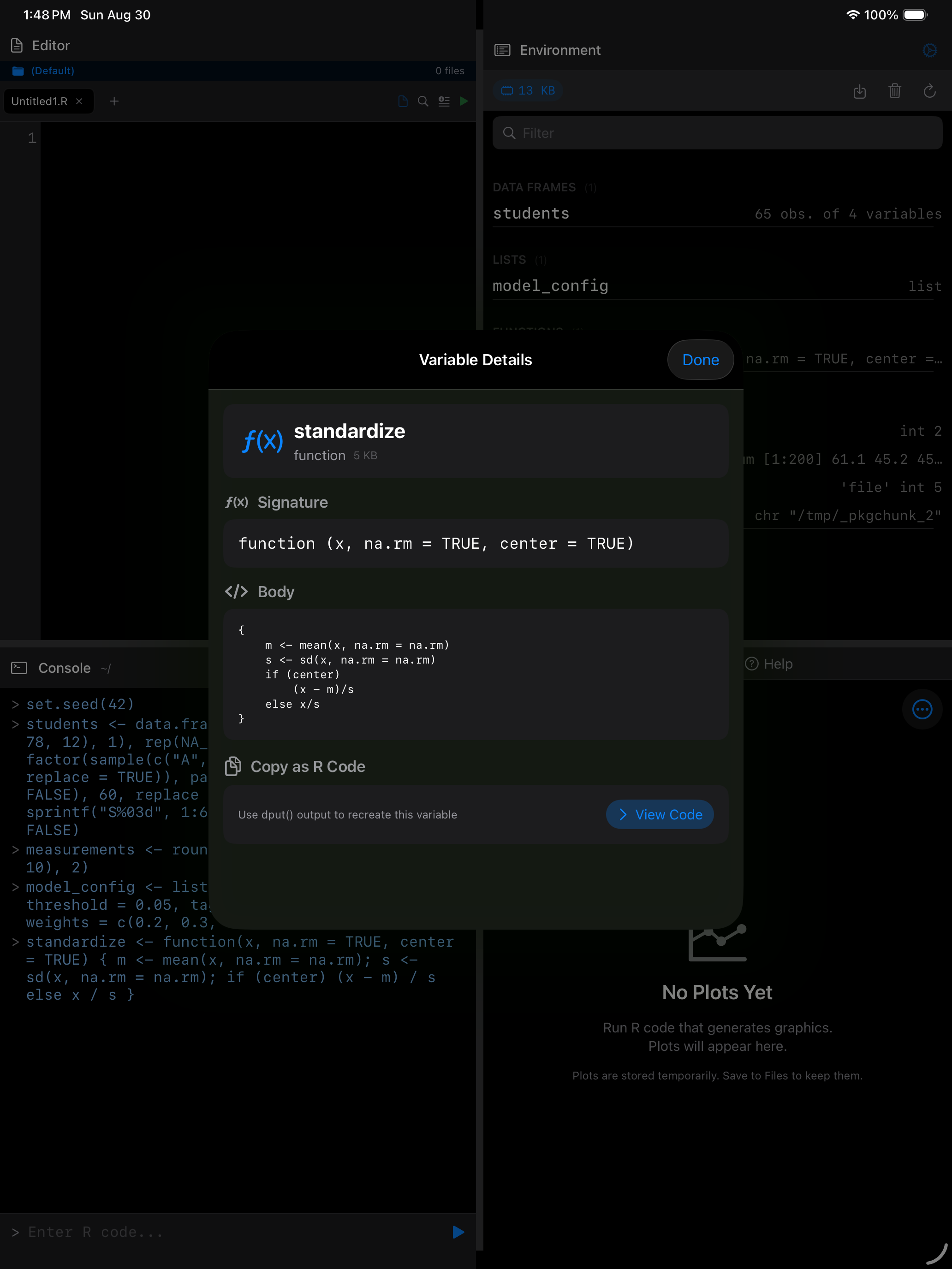
What you are seeing above: the Variable Details sheet adapts to the type of variable you tap.
- Data frame: every column with its type and sample values, plus a preview of the first rows
- Numeric vector: a summary and the first elements
- List: the
str()-style structure and a preview of each element - Function: the function’s signature (arguments) and its body
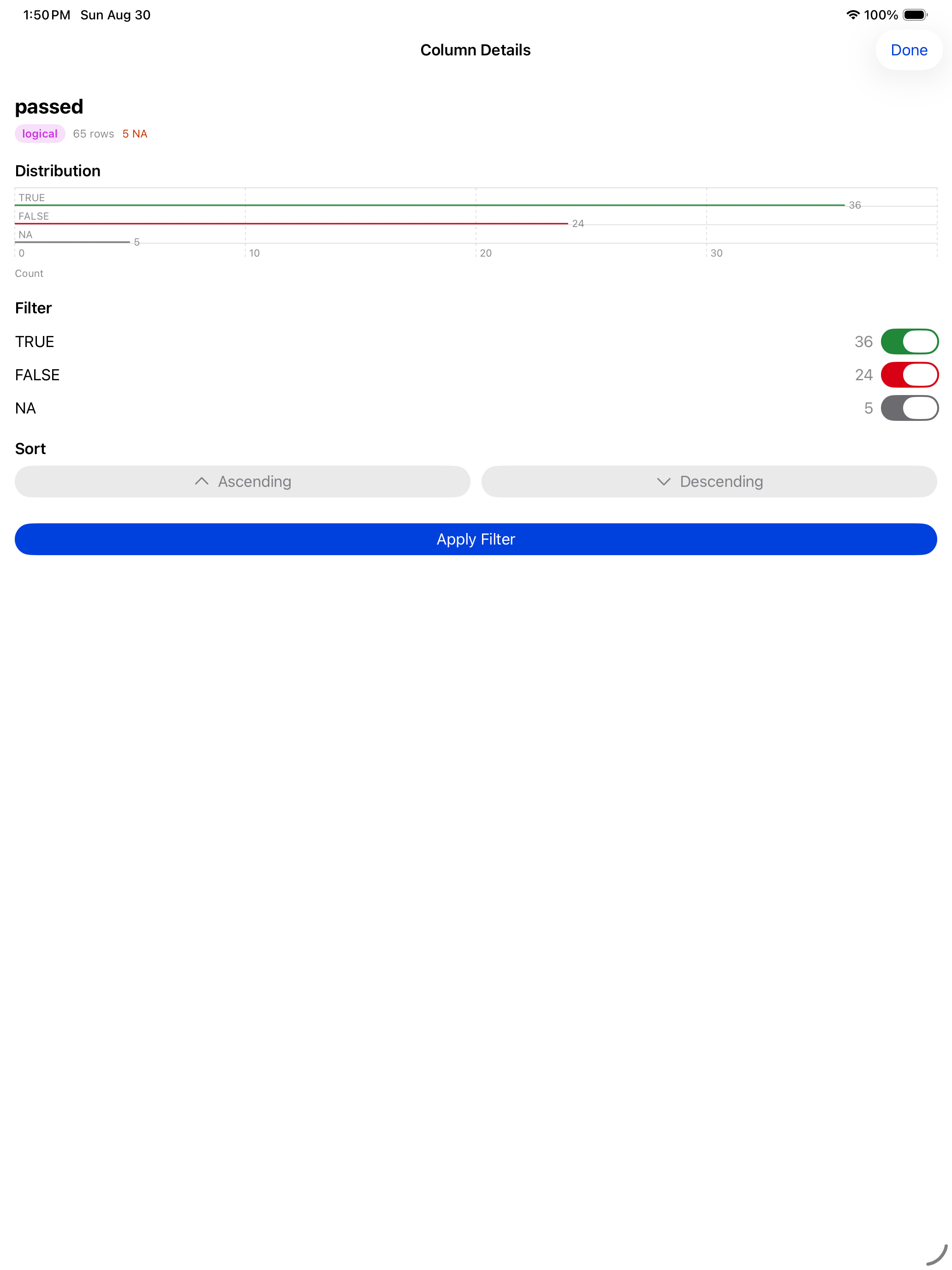
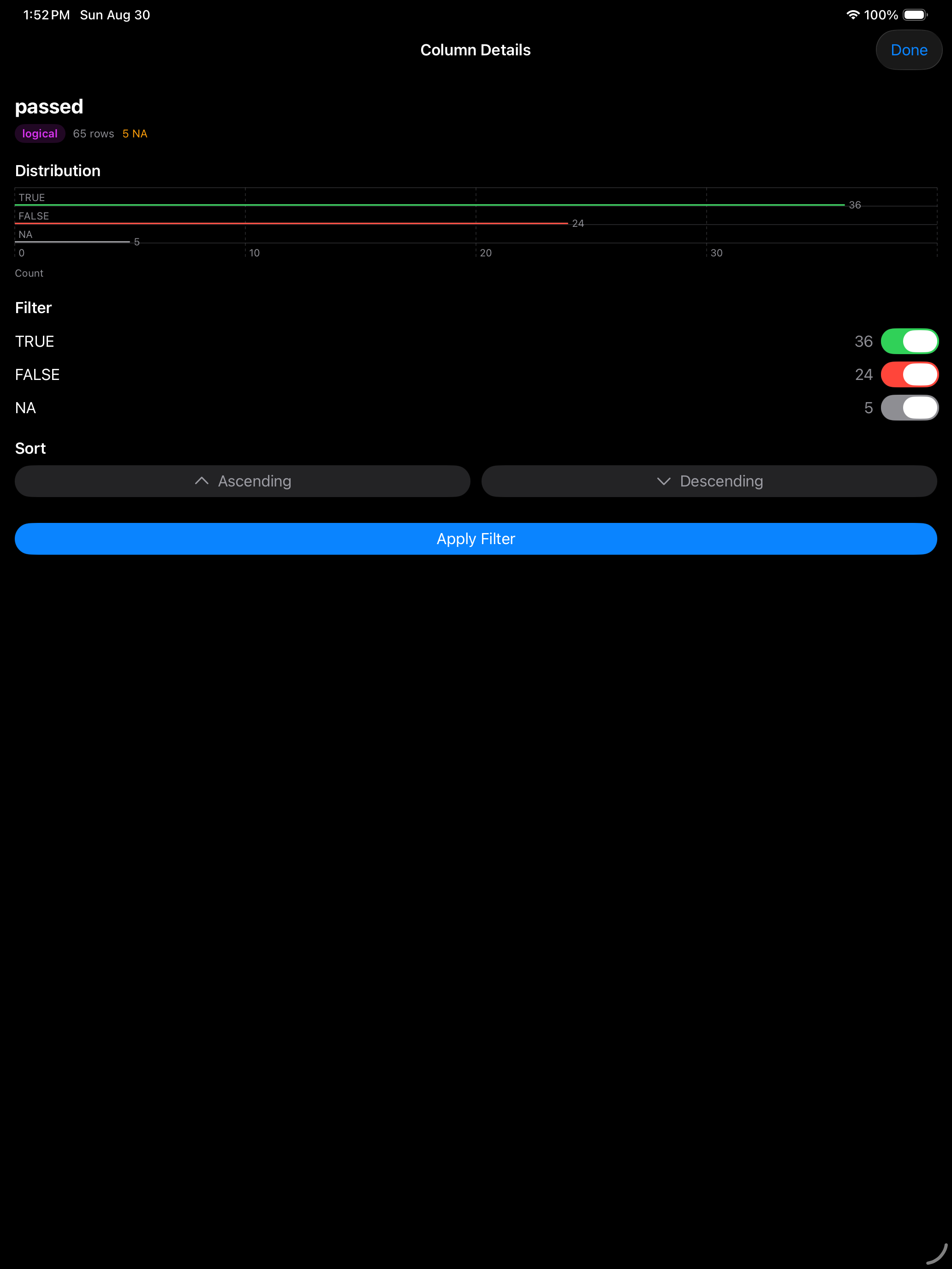
Column details
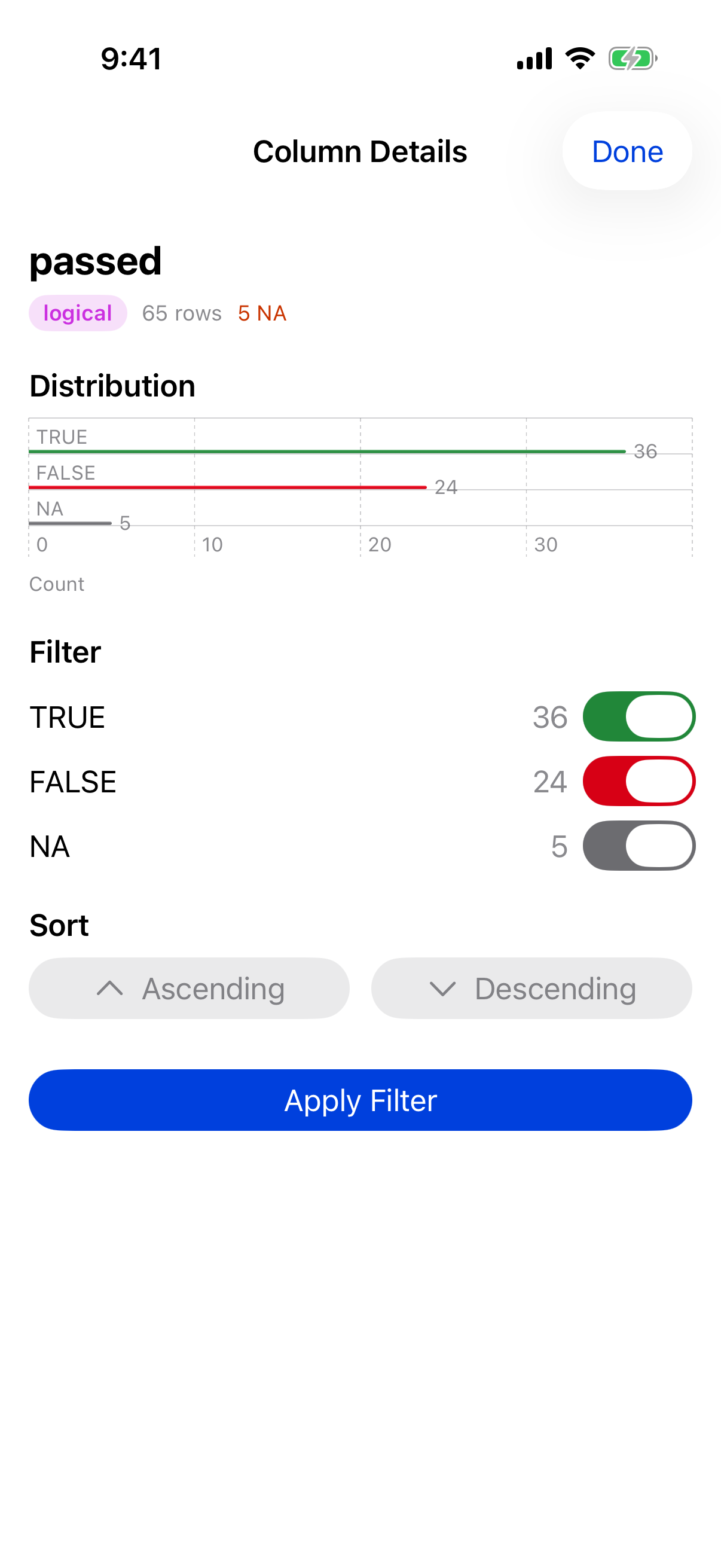
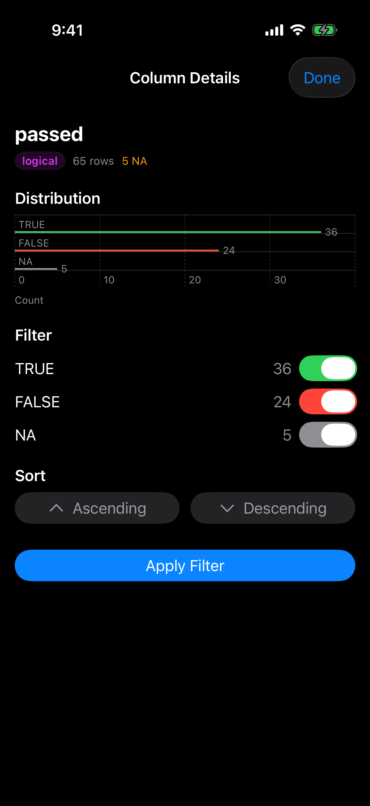
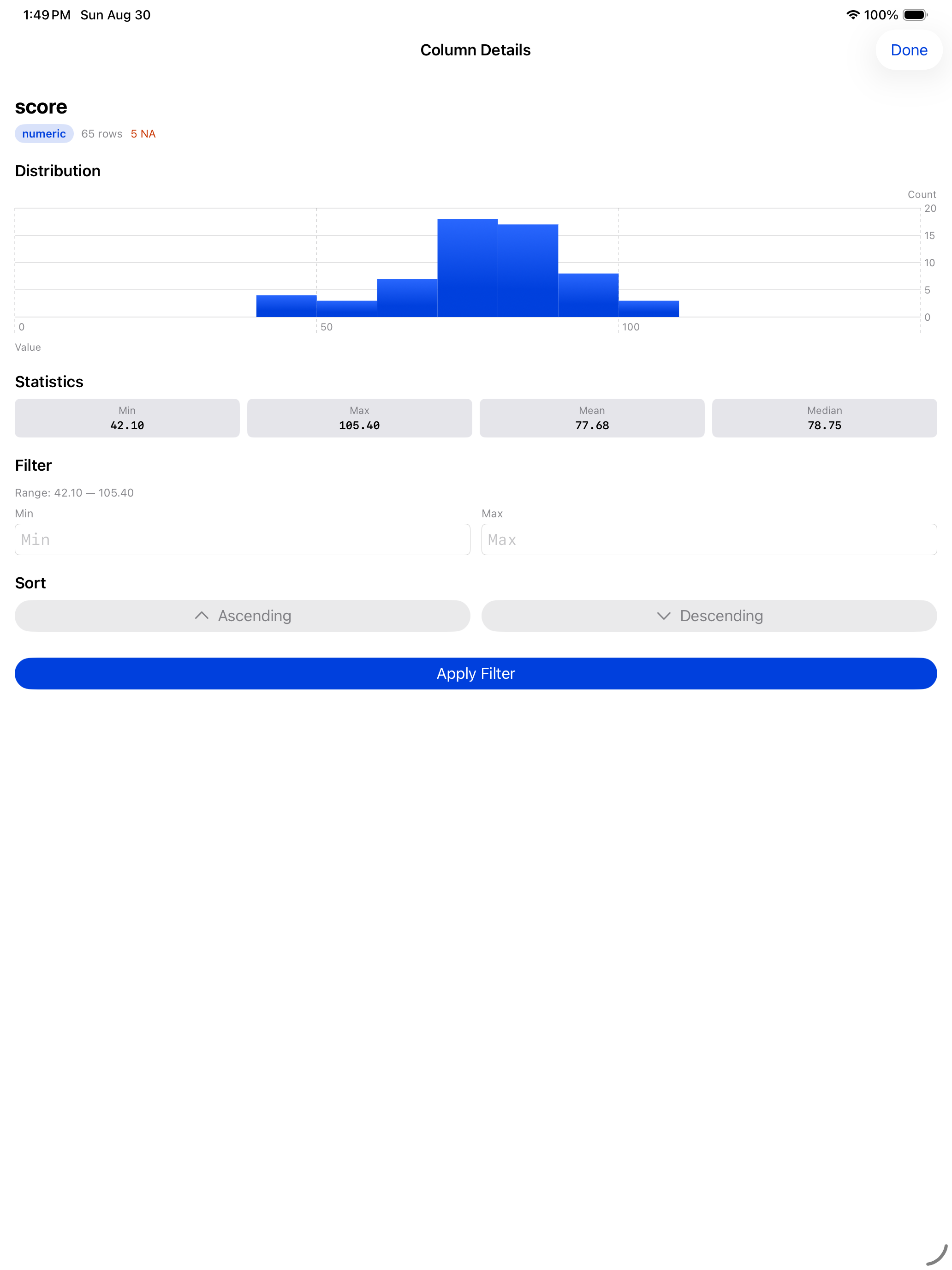
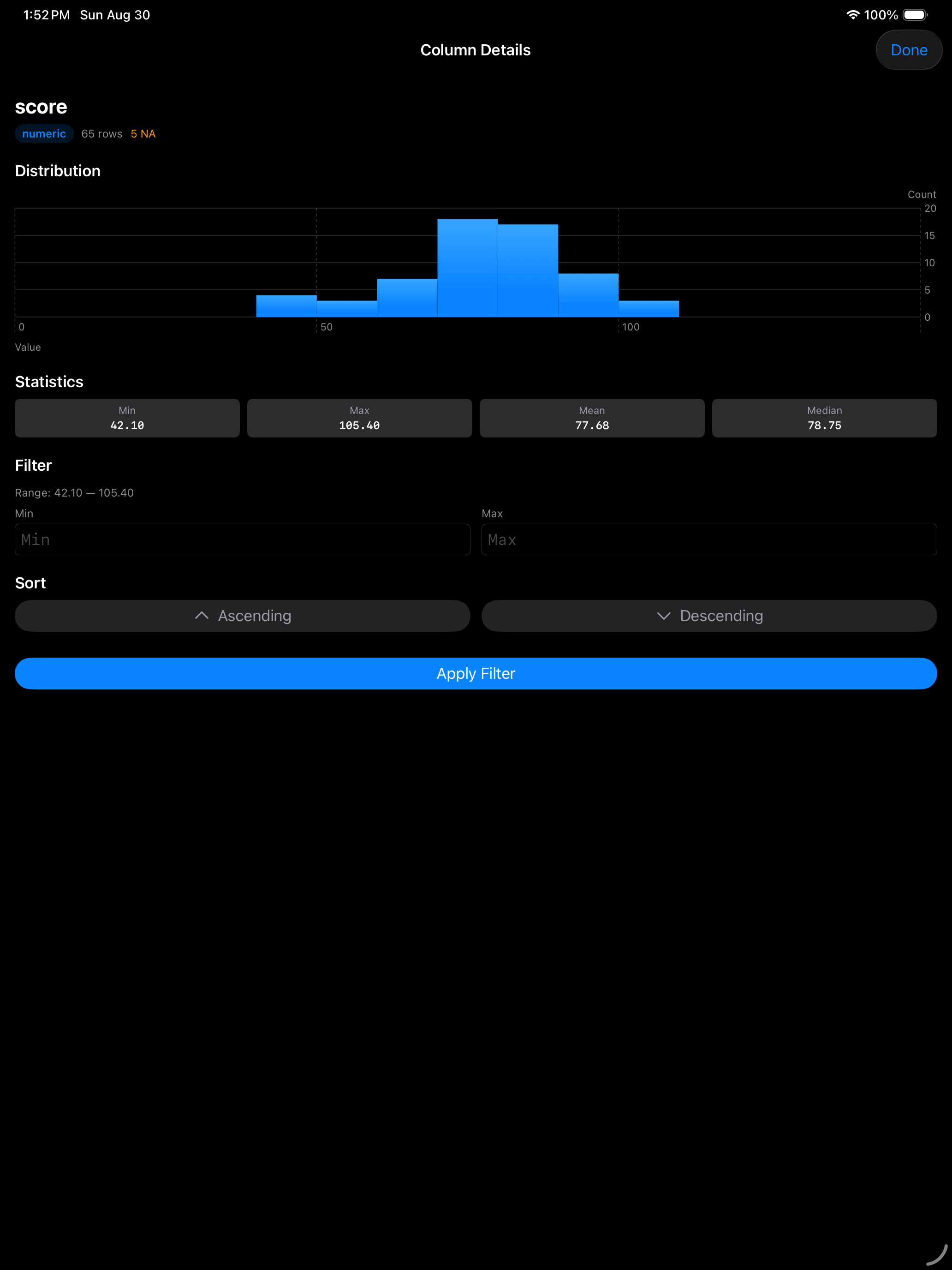
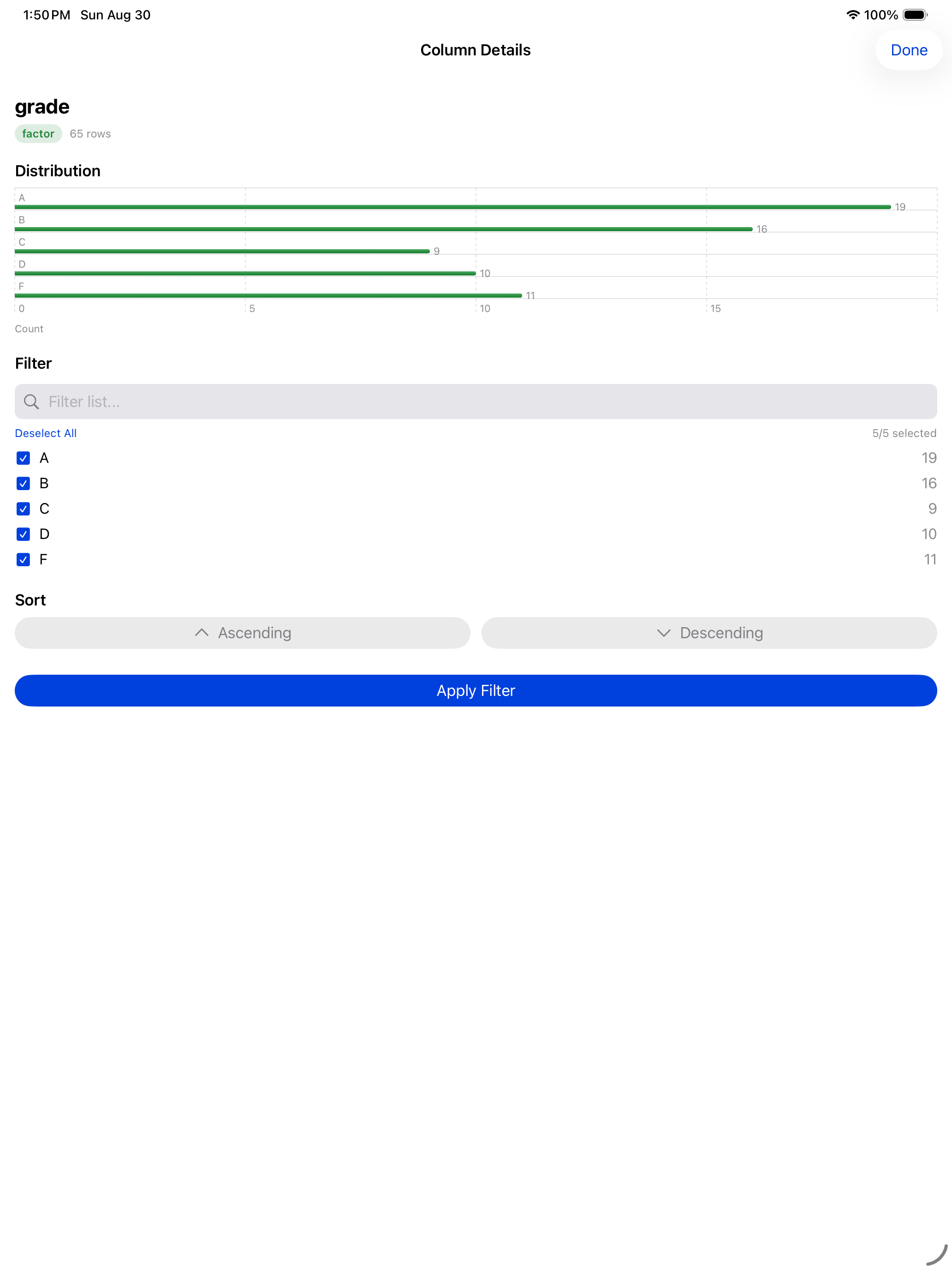
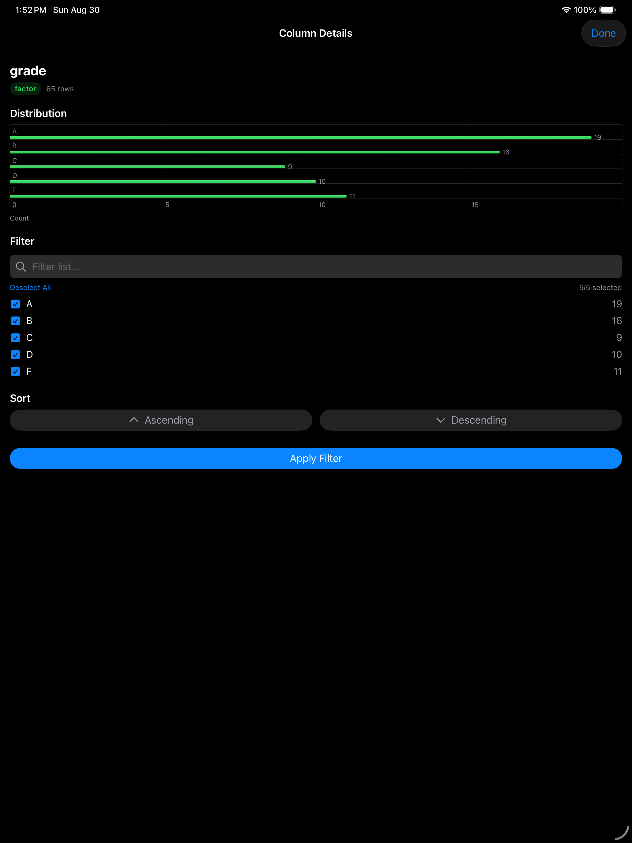
In the Data Frame Viewer, tap any column header for a column detail sheet:
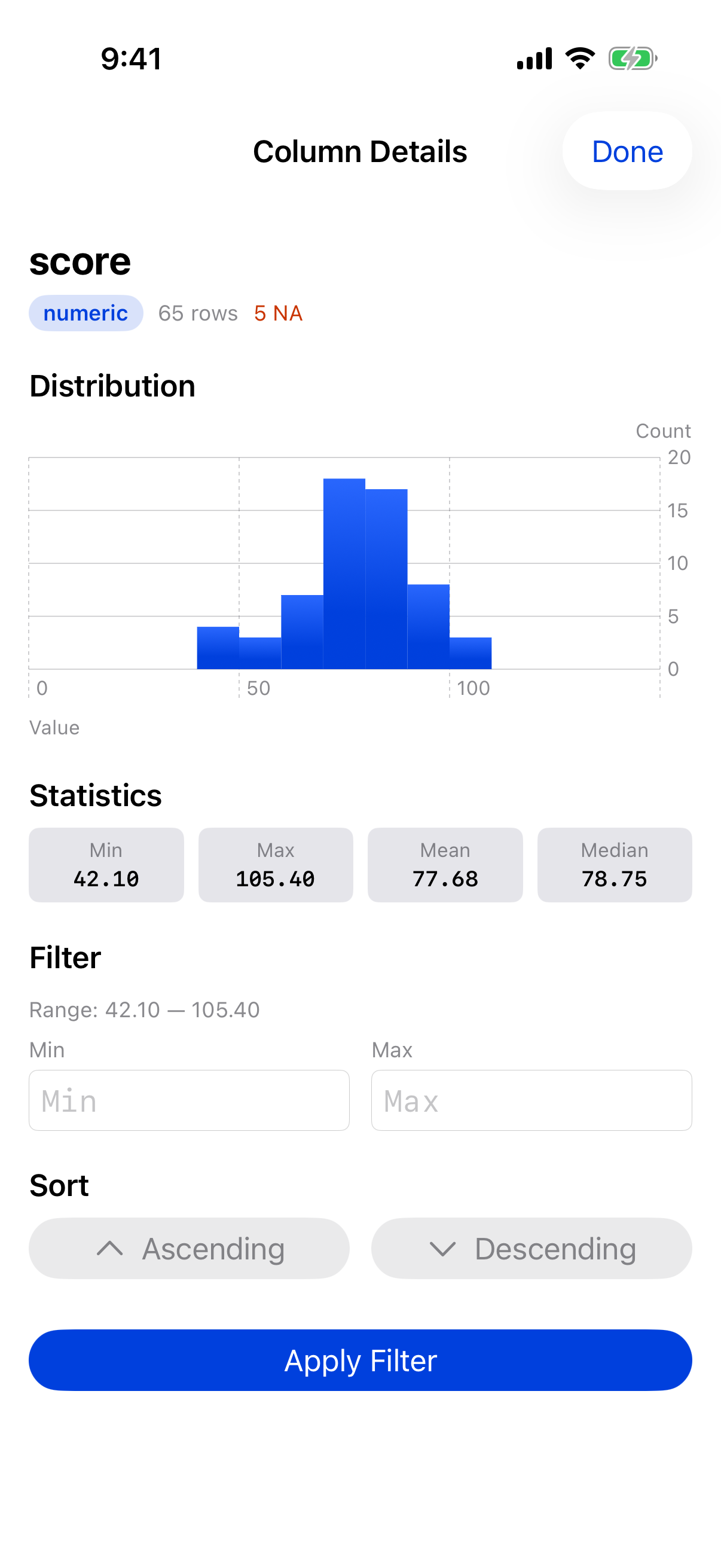
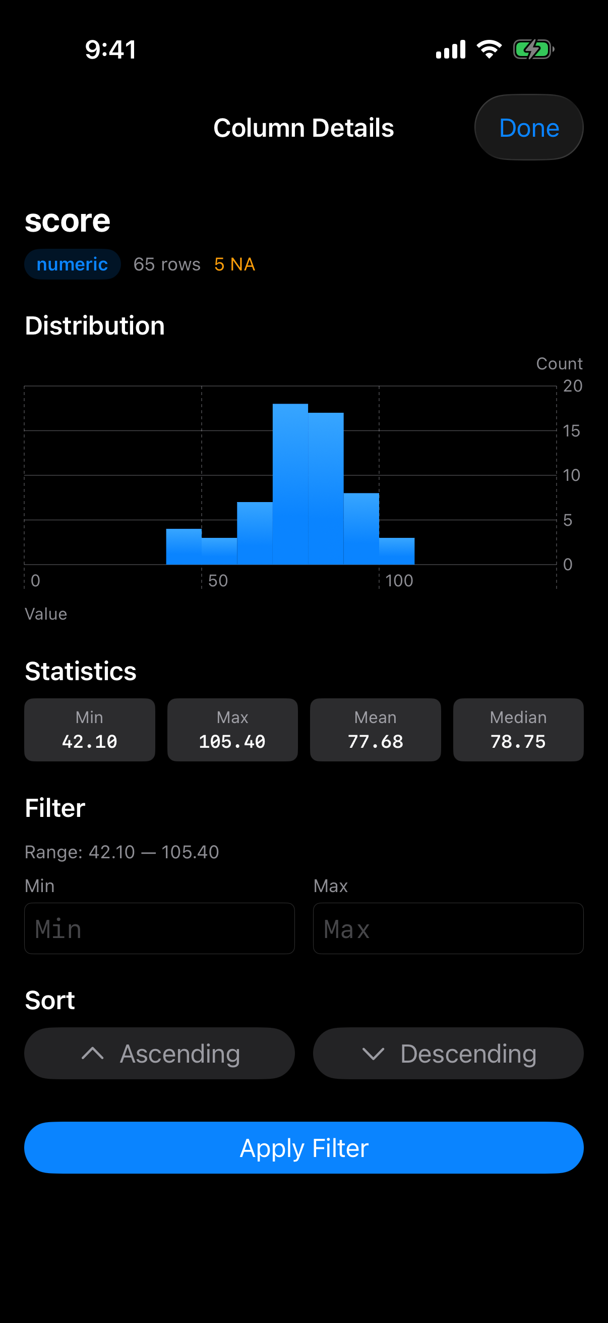
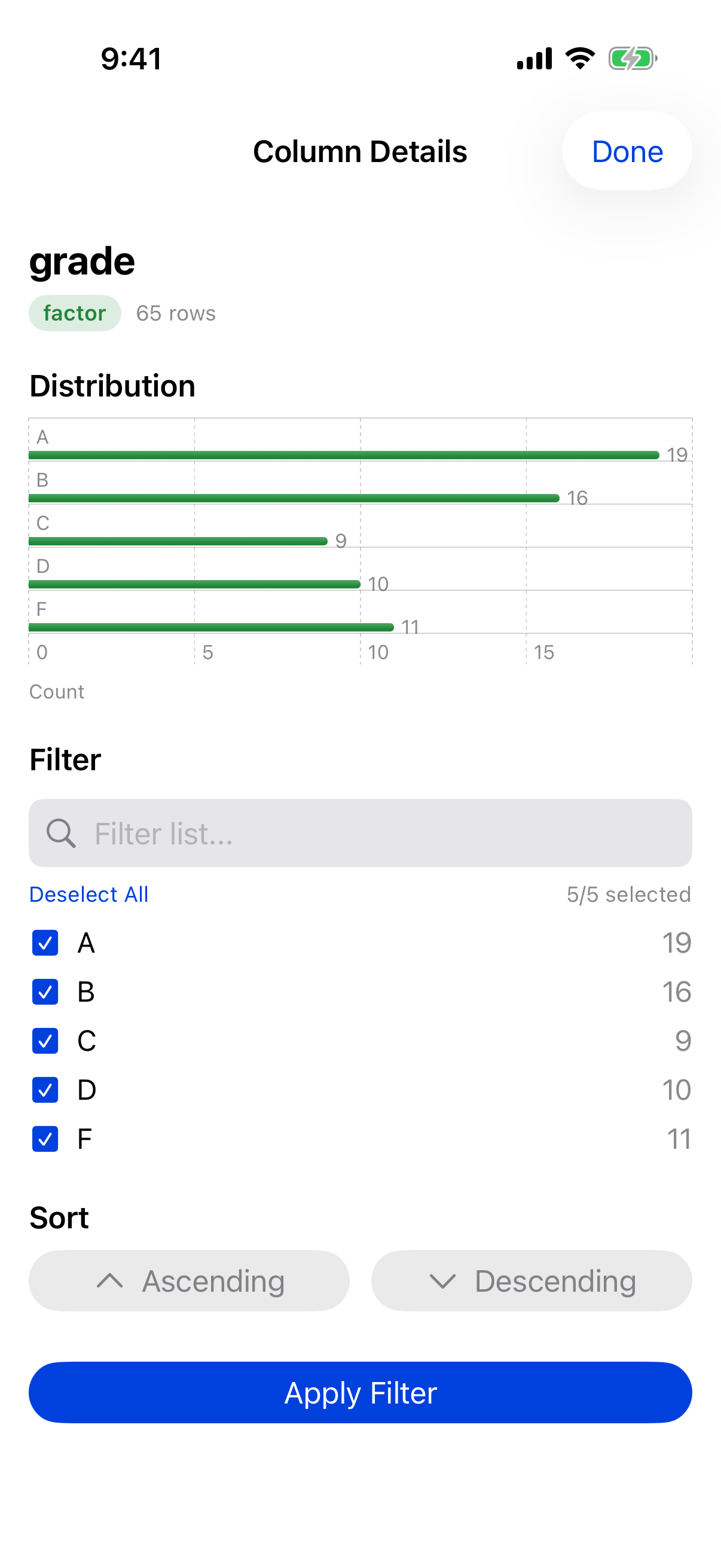
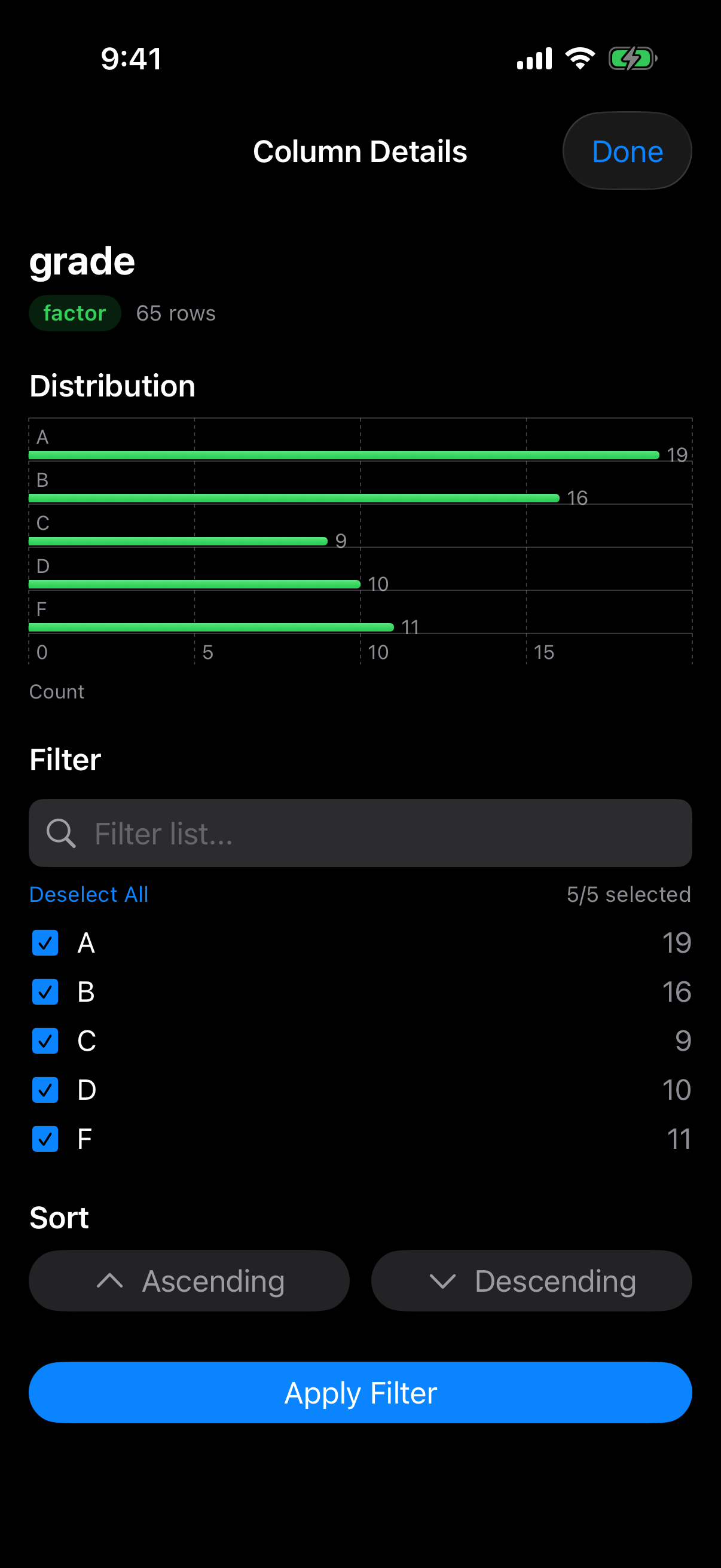
- Distribution chart: a histogram for numeric columns, a bar chart for categorical or logical columns.
- Summary statistics (numeric): min, max, mean, and median.
- Value counts (categorical): the top values and their frequencies.
- NA count: shown prominently if the column contains missing values.
Filtering and sorting
The column detail sheet also lets you filter and sort directly:
- Numeric columns: set a min/max range to filter rows. Negative numbers and your locale’s decimal separator work; Apply Filter stays disabled until the range is valid
- Categorical columns: search values and check/uncheck which ones to keep, with “Select All” and “Deselect All” buttons
- Logical columns: toggle which values to show (TRUE, FALSE, NA)
- Sort controls: tap ascending or descending to reorder the entire data frame by that column
Tap Apply Filter to update the Data Frame Viewer with your selections. Filters and sorts are applied together, making it easy to zero in on the rows that matter.
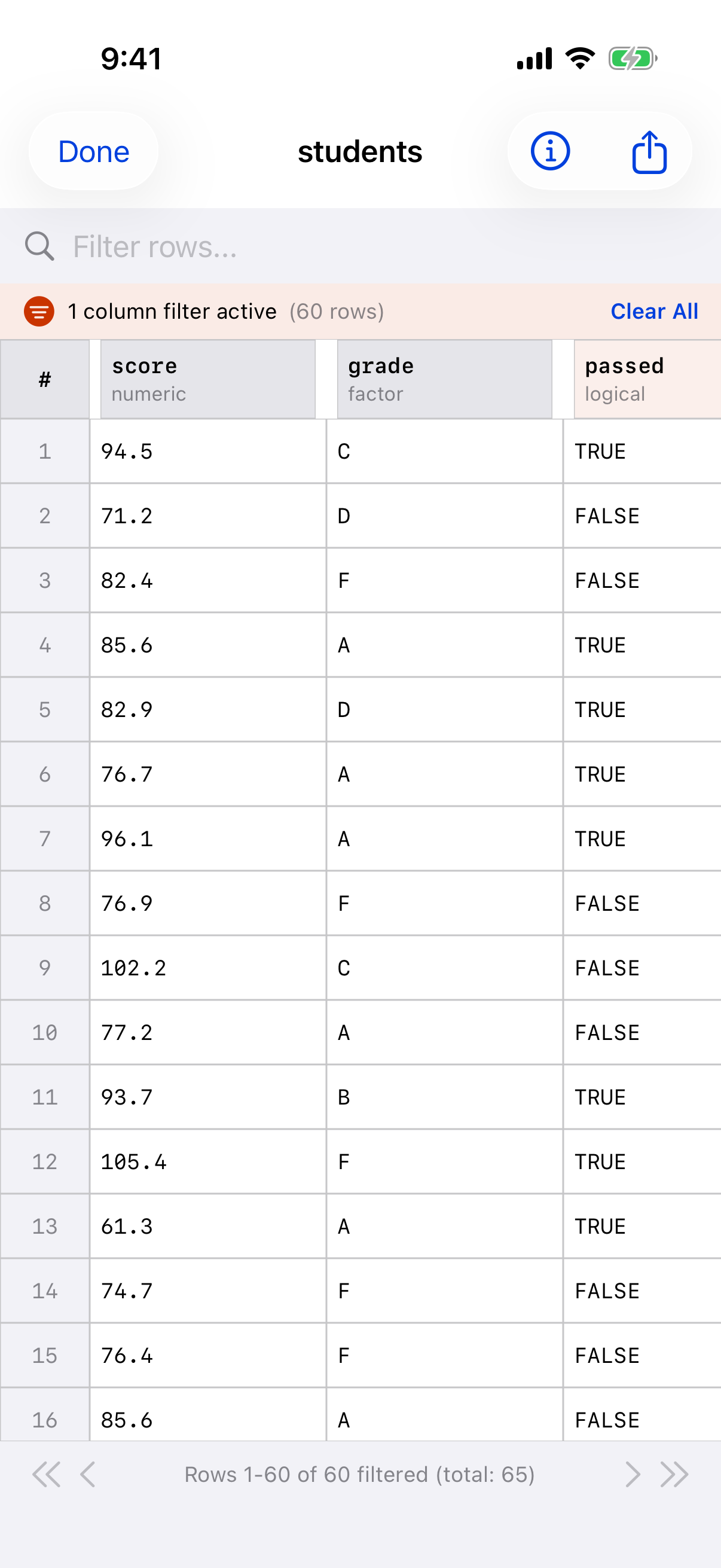
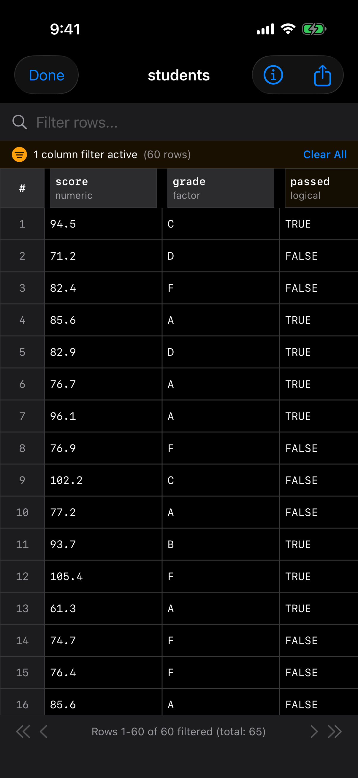
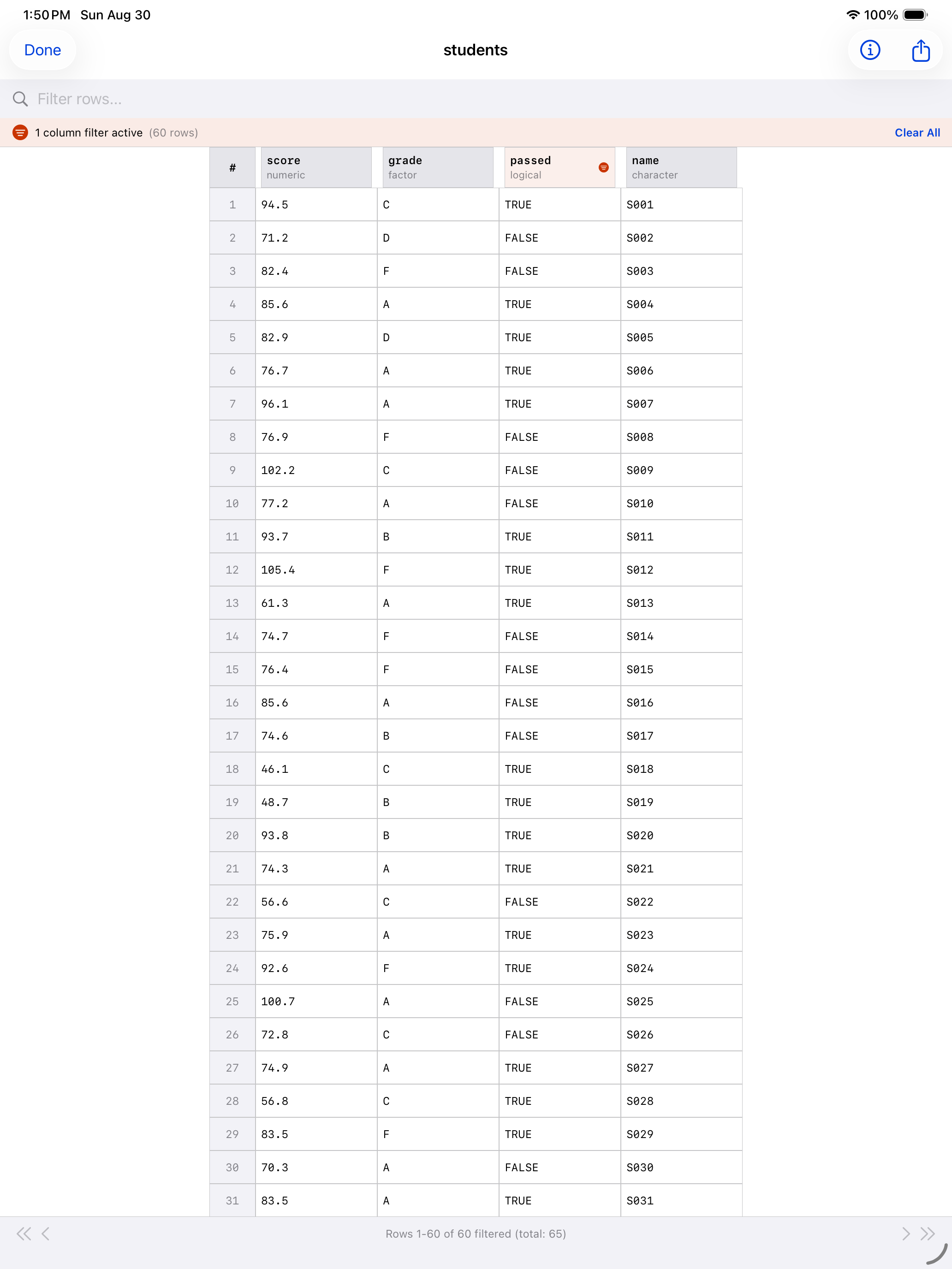
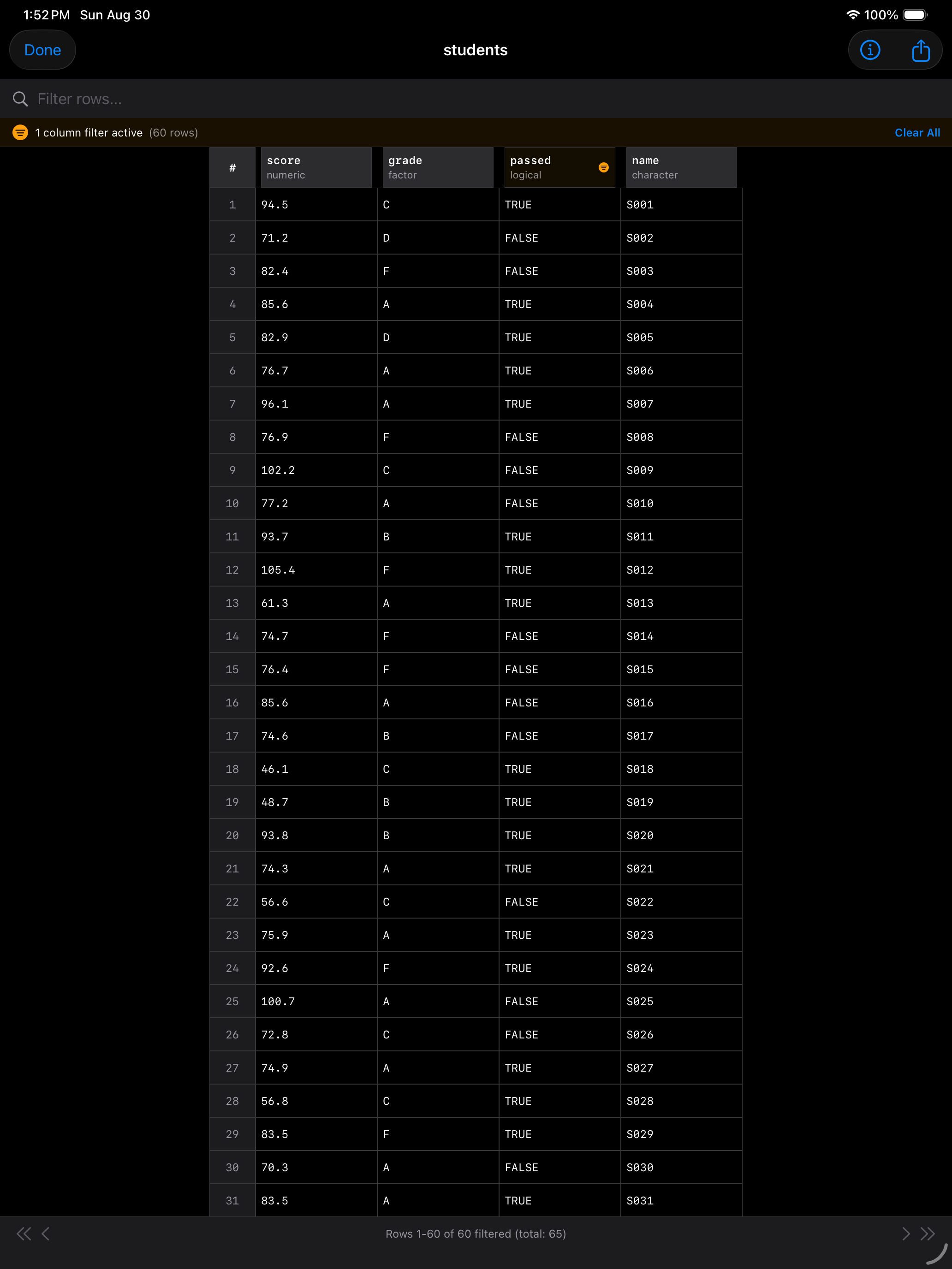
R does the filtering, sorting and searching, a page of 100 rows at a time, so even large data frames open quickly. Because the sort is R’s own order(), a text column that holds numbers sorts as text: “10” comes before “9”. Convert the column with as.numeric() if you want numeric order. A “Loading rows” indicator appears if R takes a moment, and if a page fails to load you can retry it.
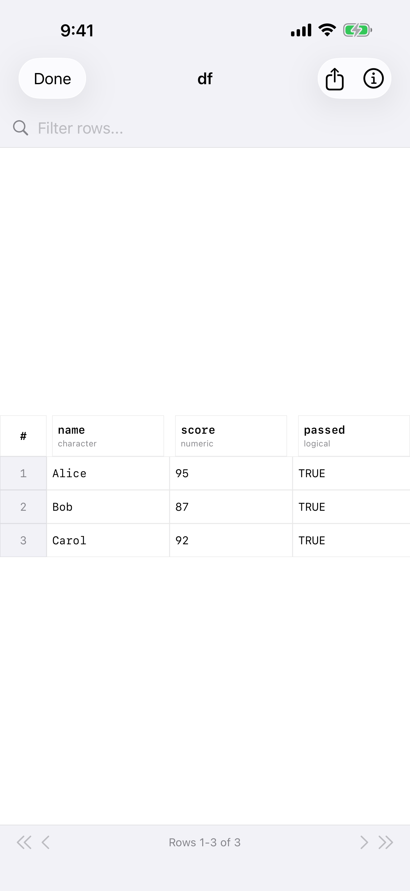
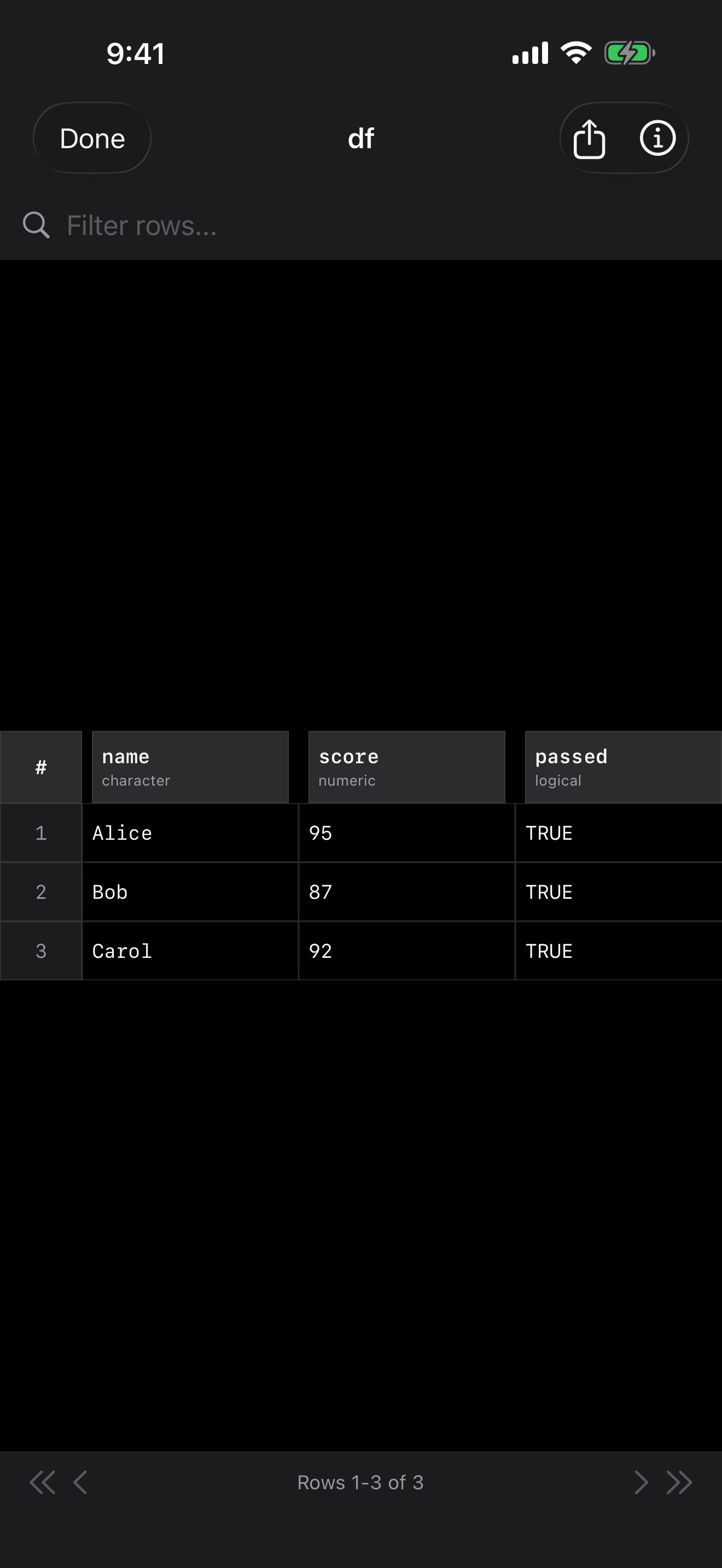
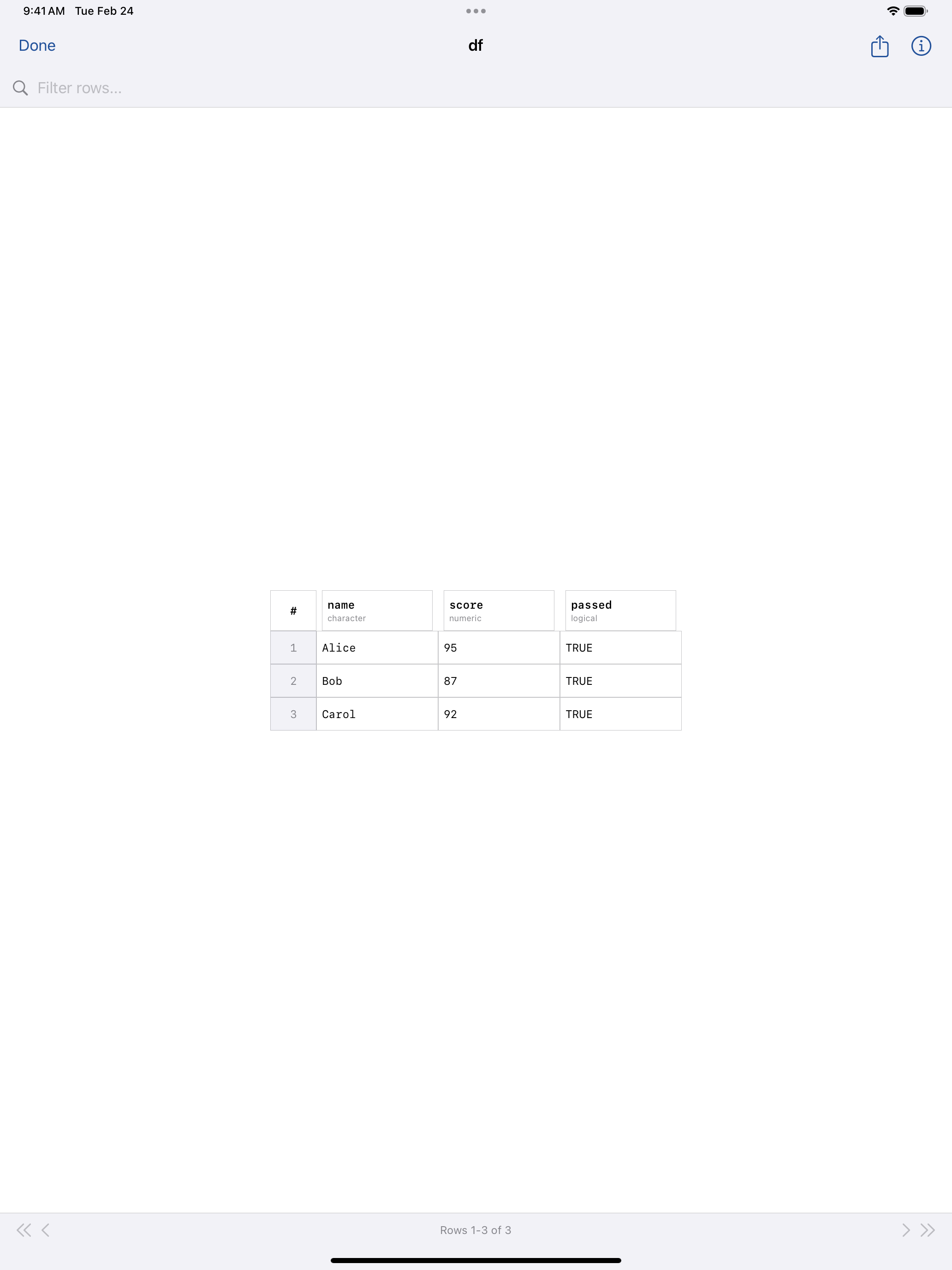
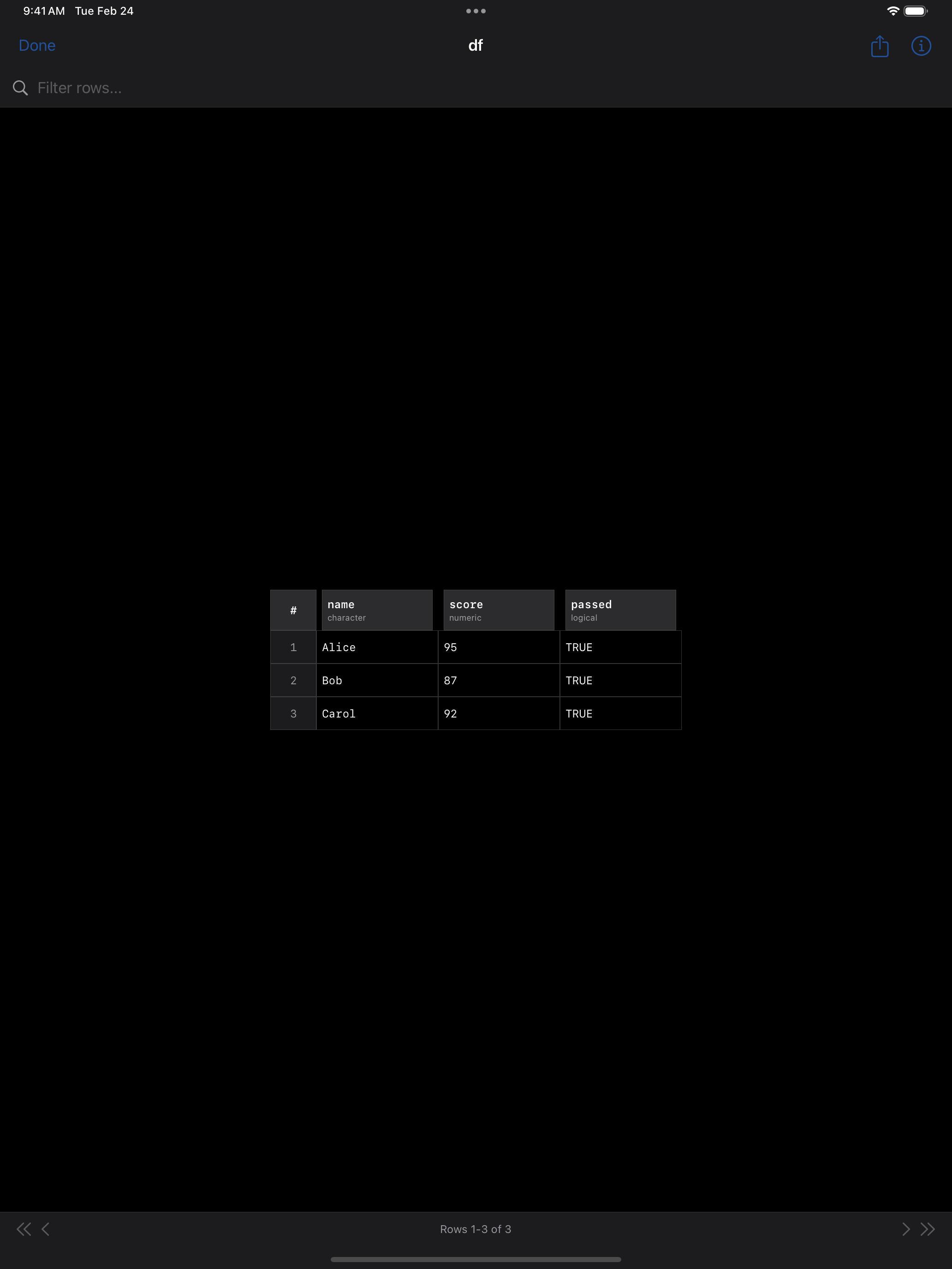
The Data Frame Viewer
- Row names: a data frame with row names of its own shows them in the first column, so
mtcarslists its cars. Otherwise the first column shows each row’s number in the data frame, which stays with the row when you filter or sort. - Search: the search box finds rows whose row name or any cell’s text contains what you type, ignoring case. Missing values match “NA”, as the grid shows them.
- Changes in R: if the data frame’s number of rows or columns changes in R while it is open, the viewer reloads with your filters and tells you why.
- Export: tap the share button. Export as CSV saves the whole data frame into the current project’s folder and opens the share sheet (Save to Files, AirDrop, and so on). With a filter or sort applied and the search box empty, Export Current View as CSV saves only the rows shown, in their order. Copy View as R Code copies the R code that selects the same rows the grid shows.
With VoiceOver, each column header reads its name, type, sort and filter state, each cell names its row and column (“Mazda RX4, mpg, 21”), and cells offer a Copy Value action.
Comparing data frames
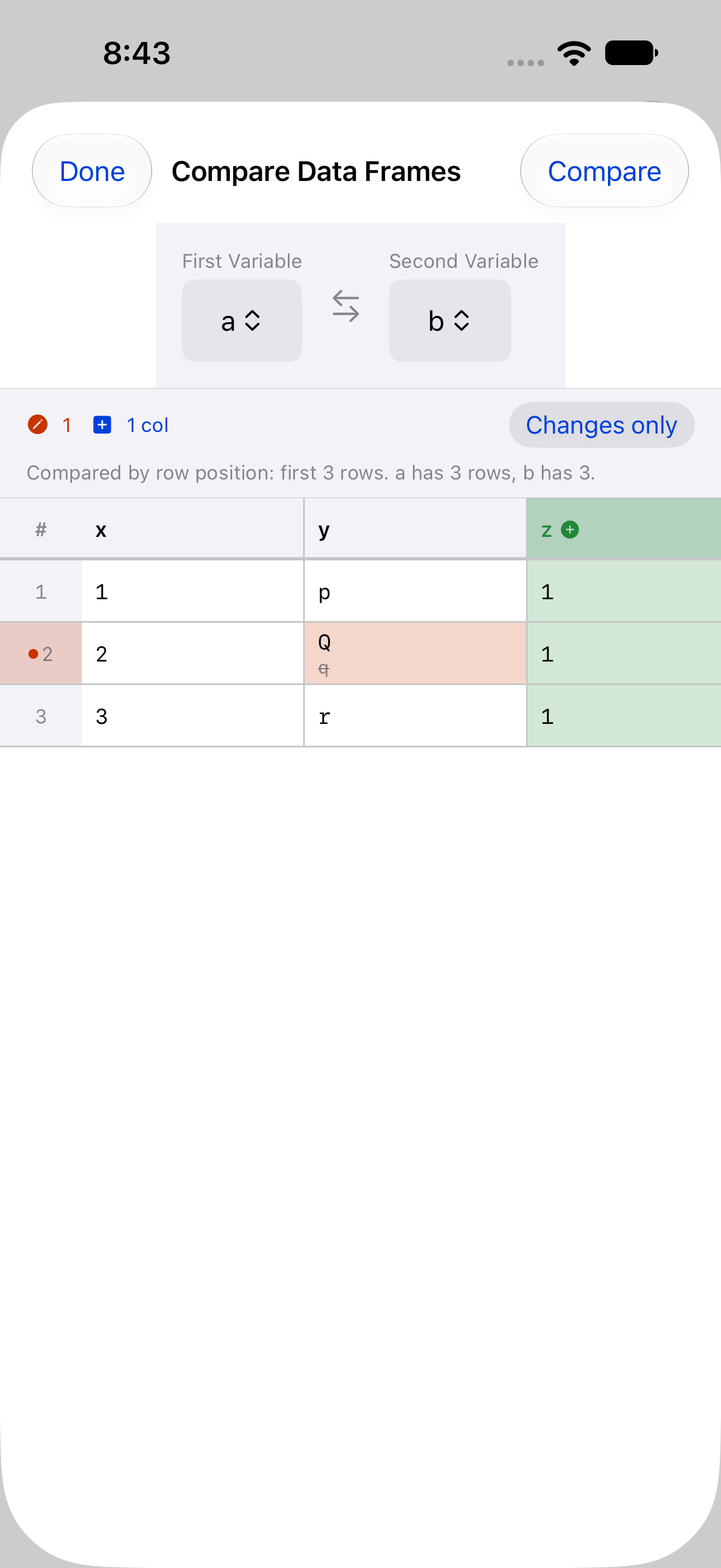
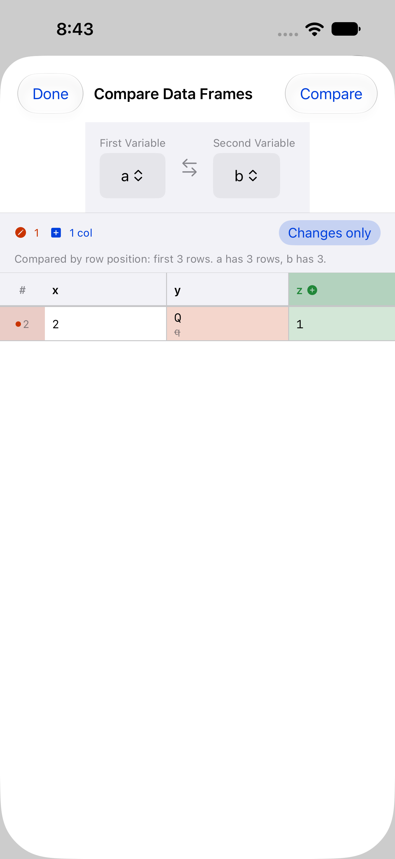
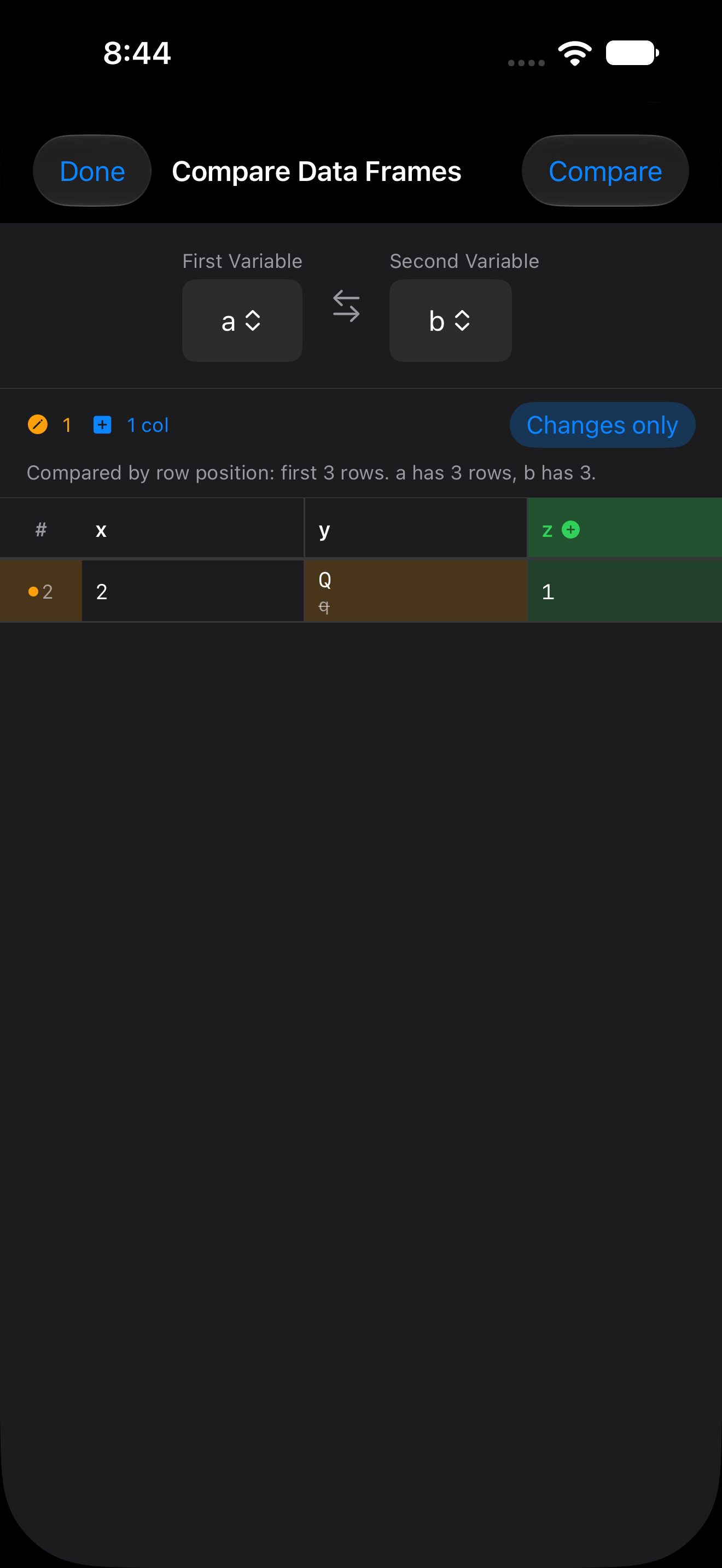
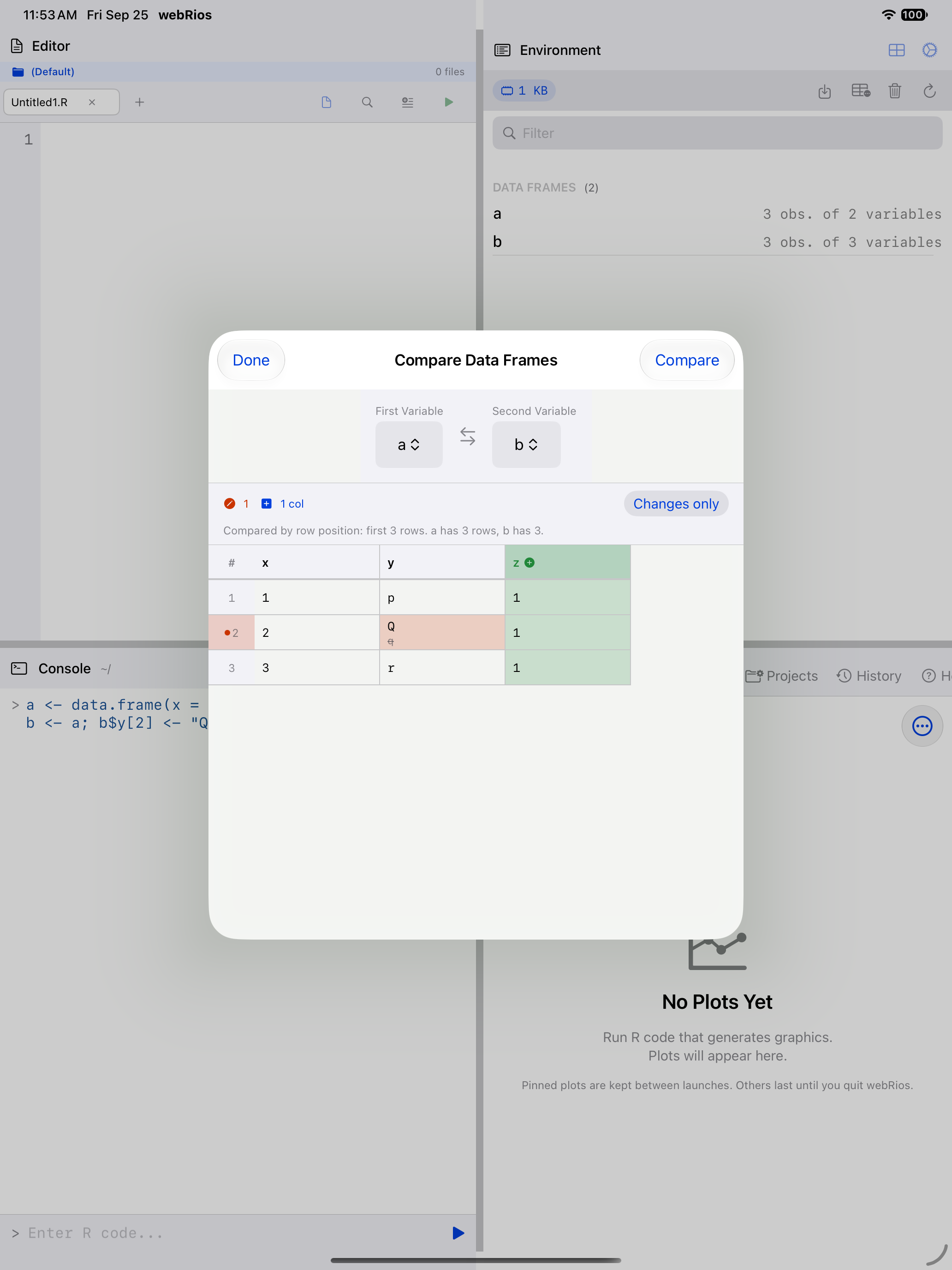
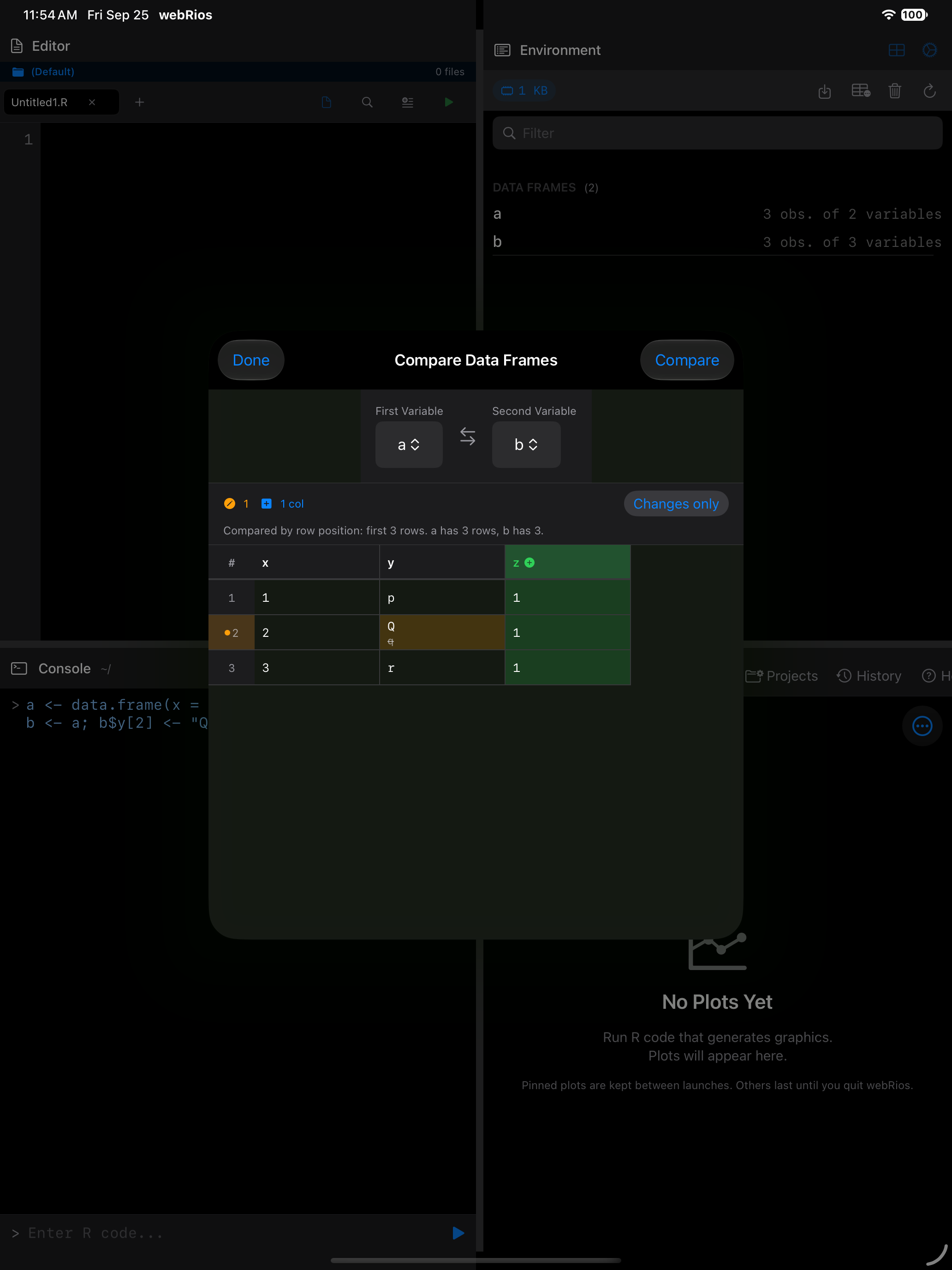
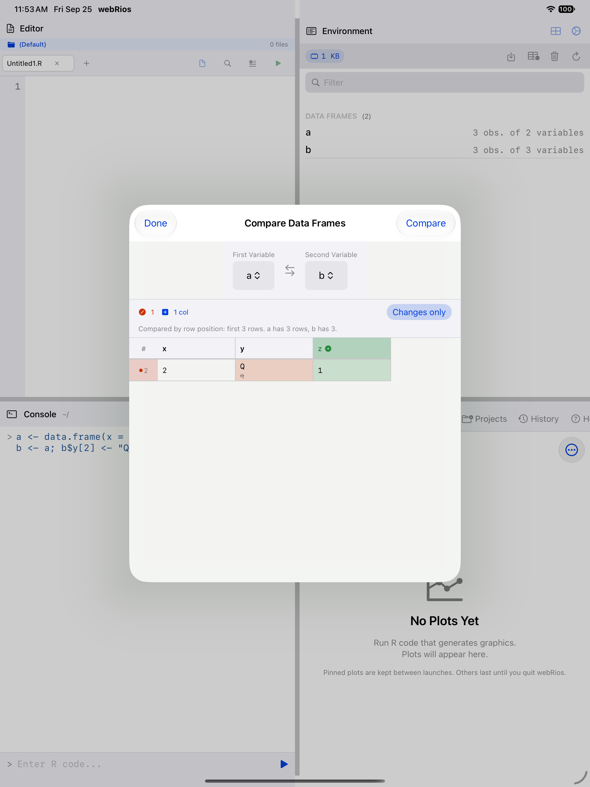
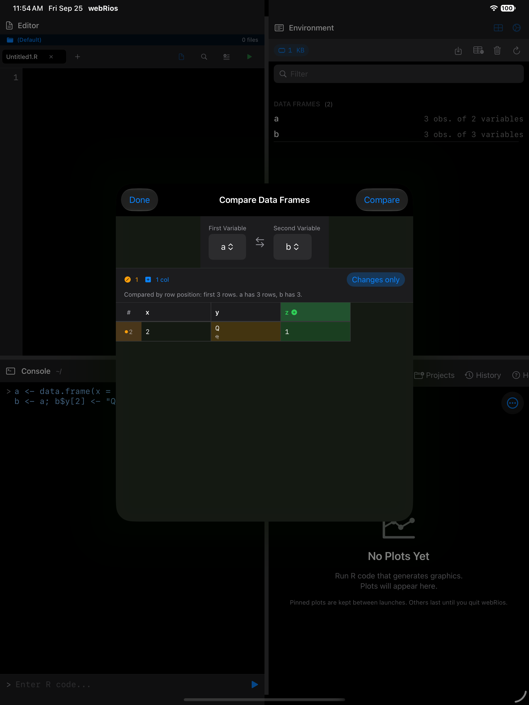
Open the Environment … menu and choose Compare Data Frames. Pick a first and a second data frame (if there are exactly two, they are already selected), then tap Compare.
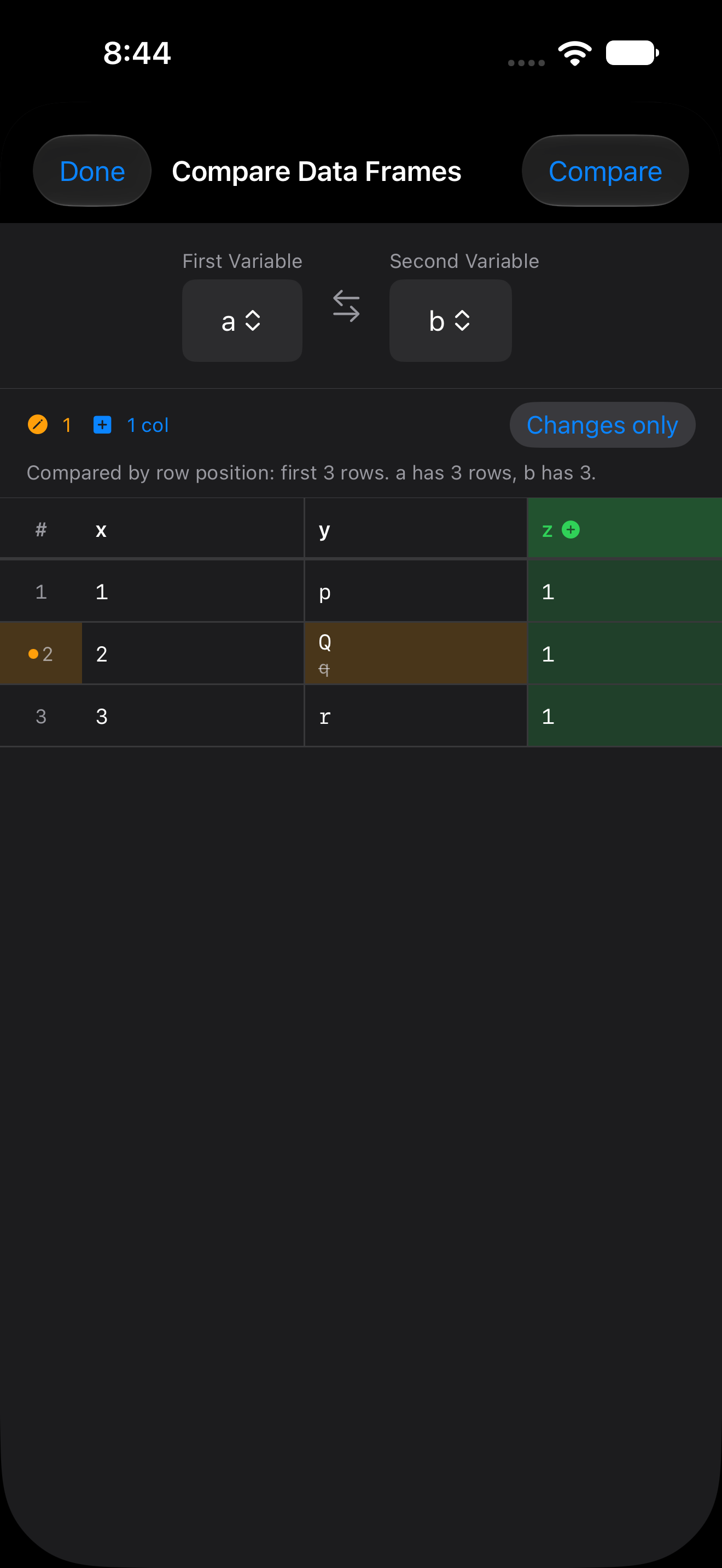
Rows are compared by position, up to the first 1,000 rows of each, and a caption says how many were compared. Columns are matched by name. Changed values show the new value over the old one struck through. Rows and columns that exist in only one data frame are marked added or removed, and a column whose type changed is flagged. Changes only hides the unchanged rows. With VoiceOver, each cell reads its row, column and what changed, for example “changed from q to Q”.
Quick actions with long press
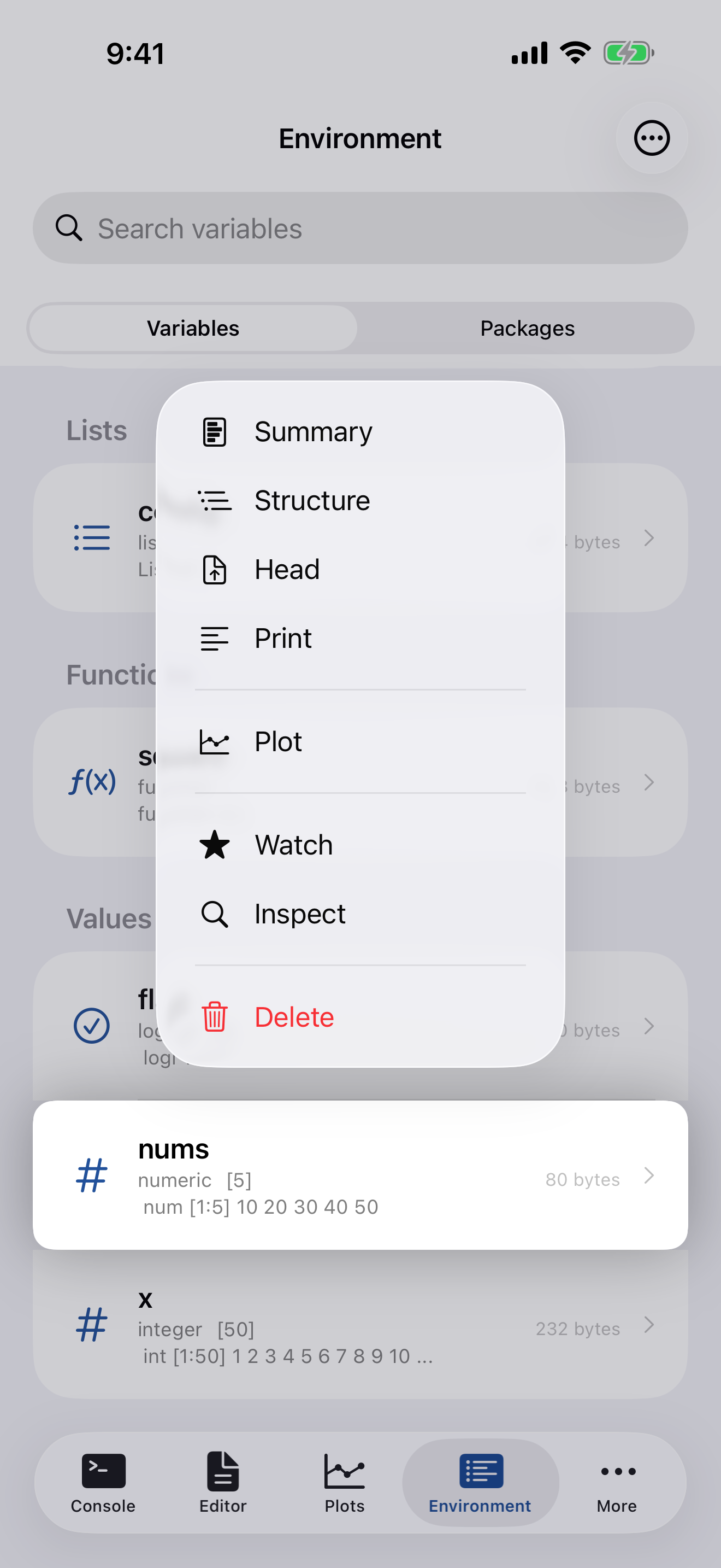
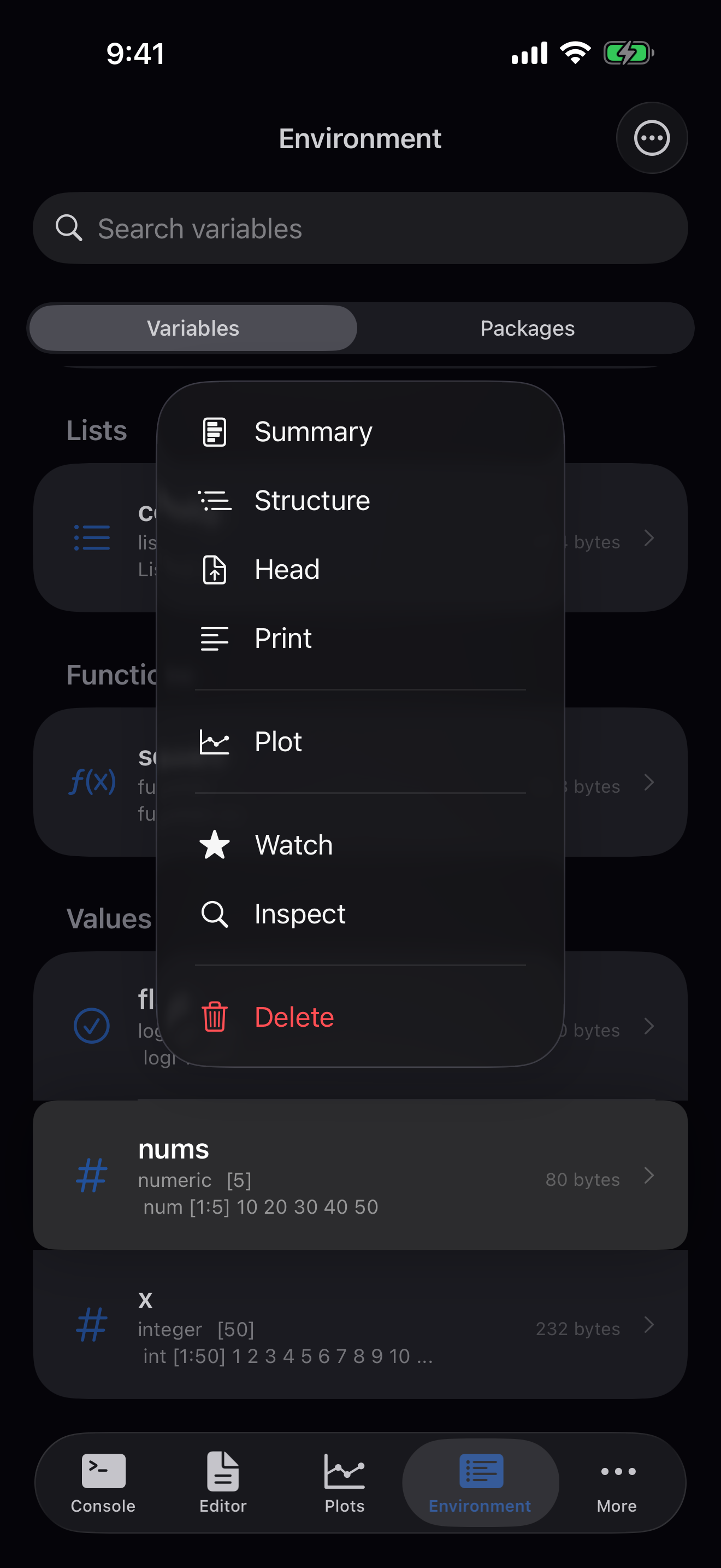
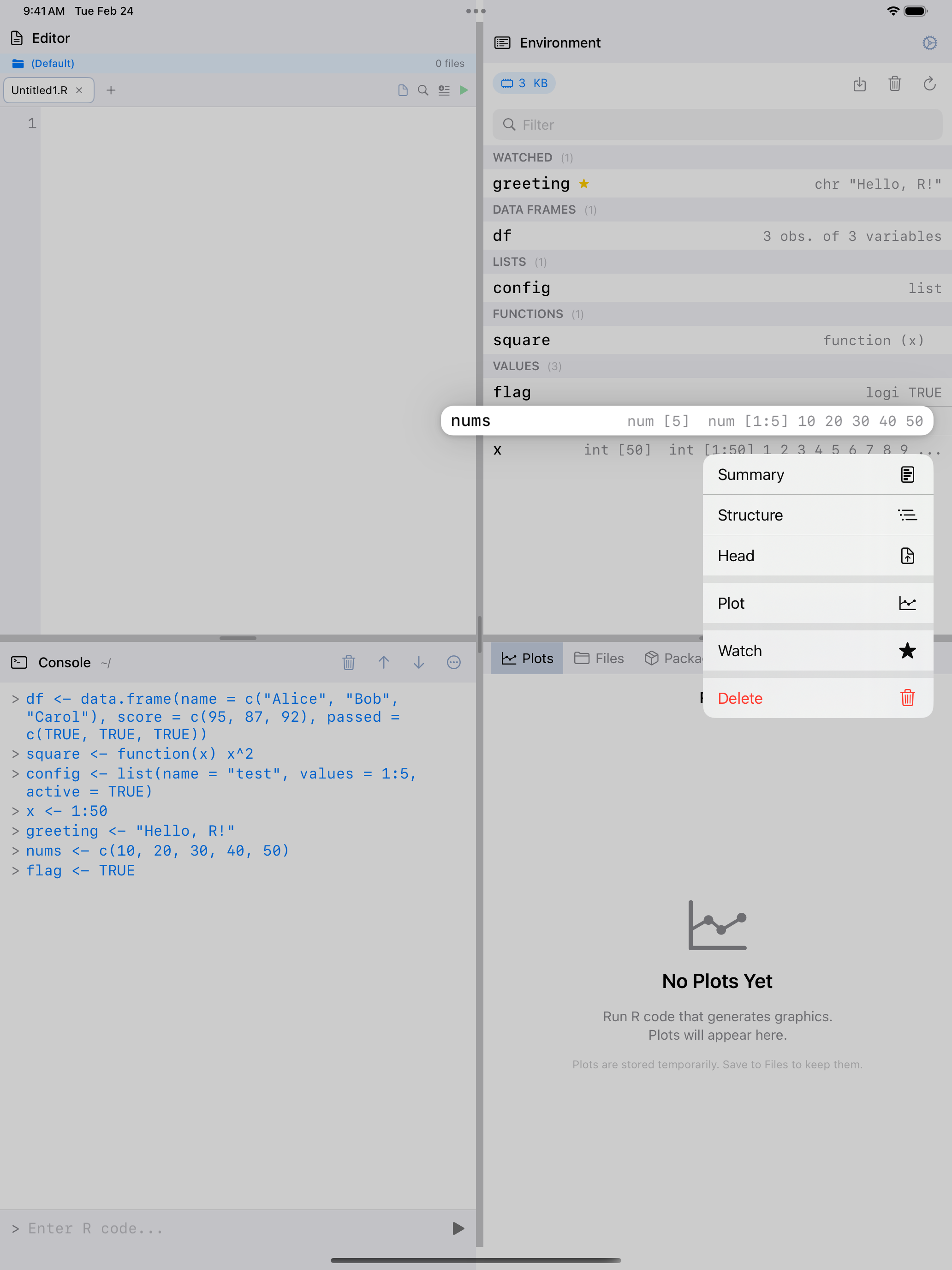
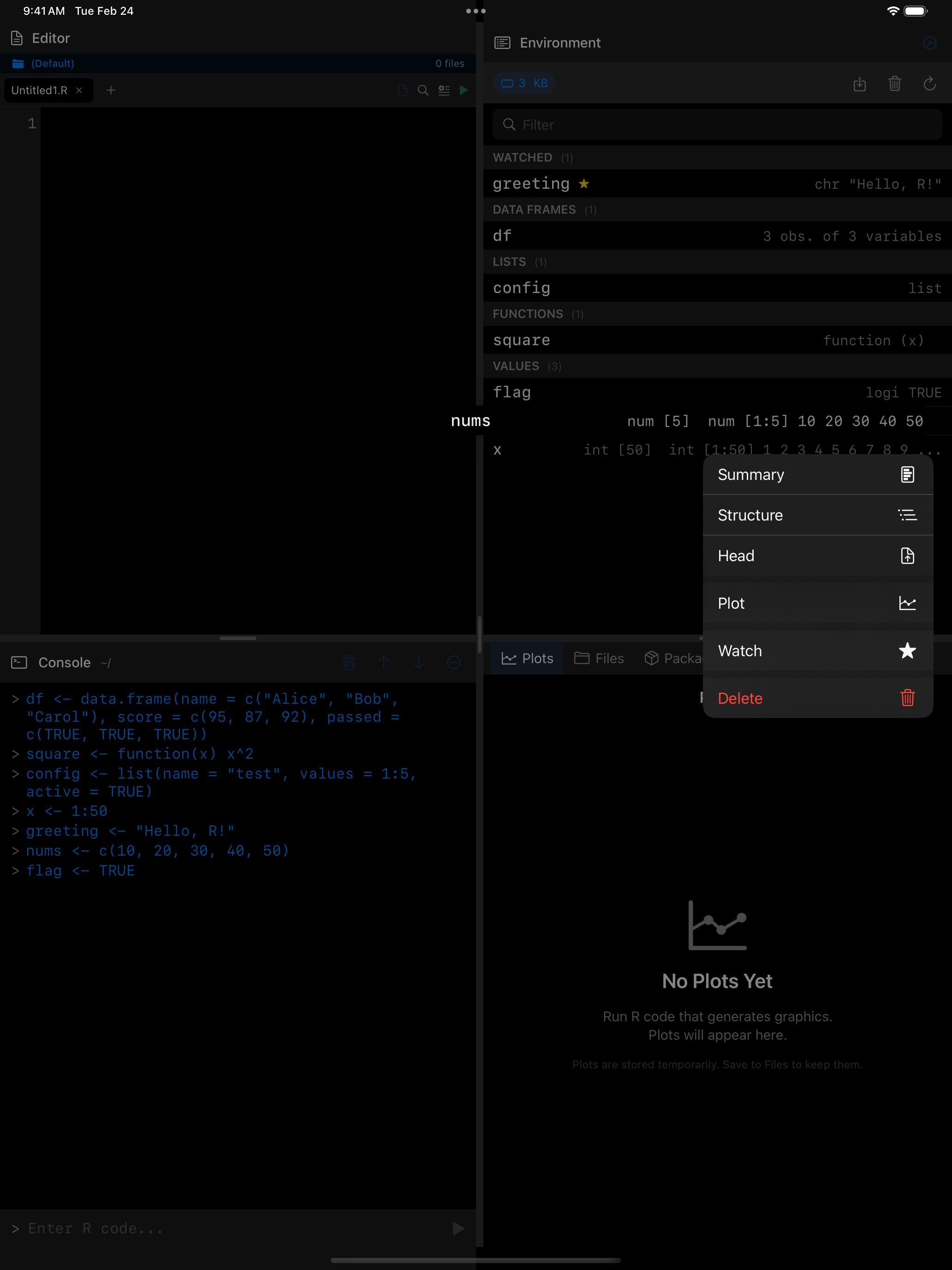
Long-press any variable (or right-click on iPad) for a context menu of quick actions:
- Summary: runs
summary()and shows the result in a popup - Structure: runs
str()so you can see the internal structure - Head: shows
head()output (the first few rows or elements) - Print: runs
print()for the full output - Plot: generates a quick plot of the variable (the plot appears in the Plots tab)
Watching variables
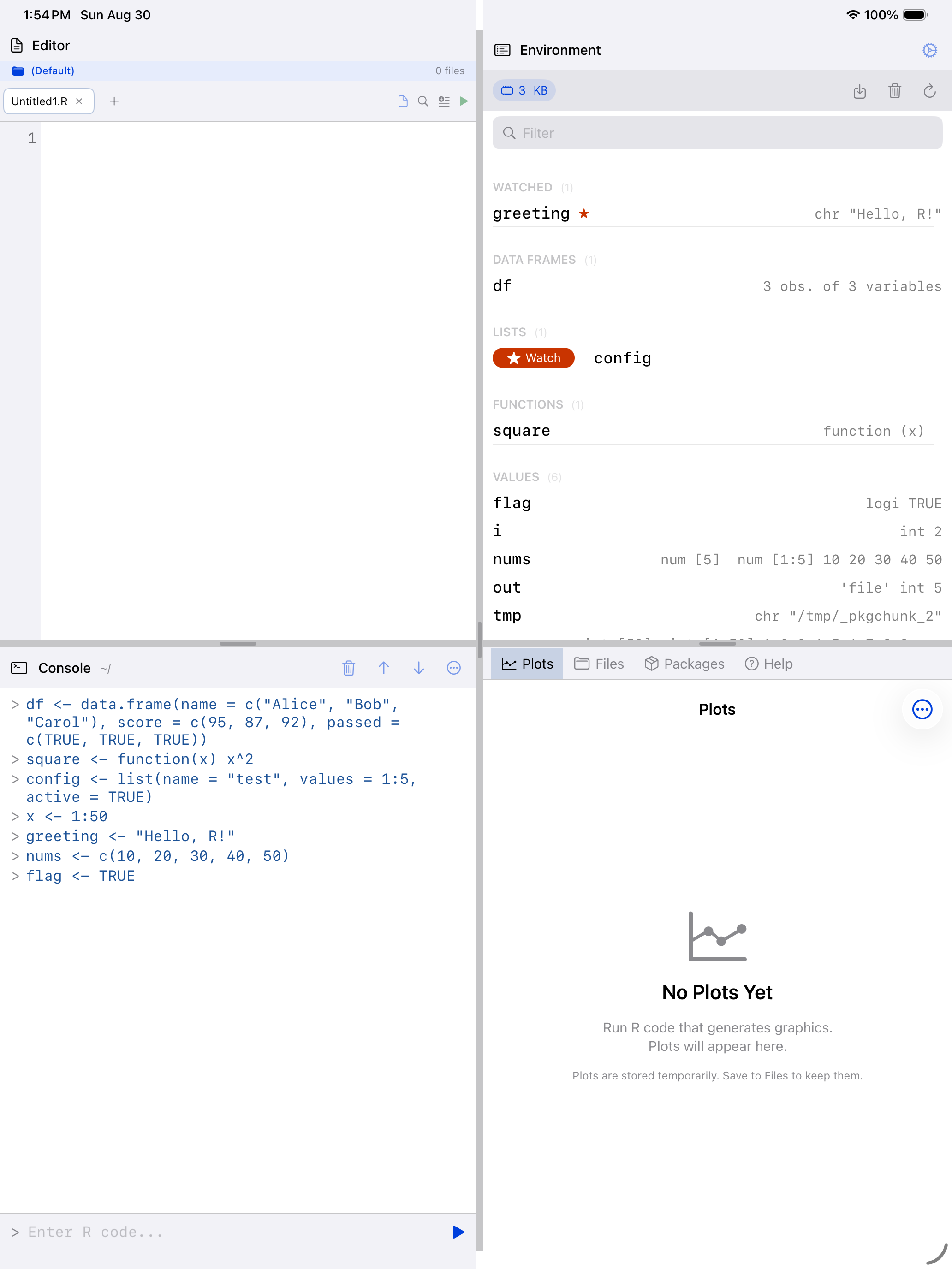
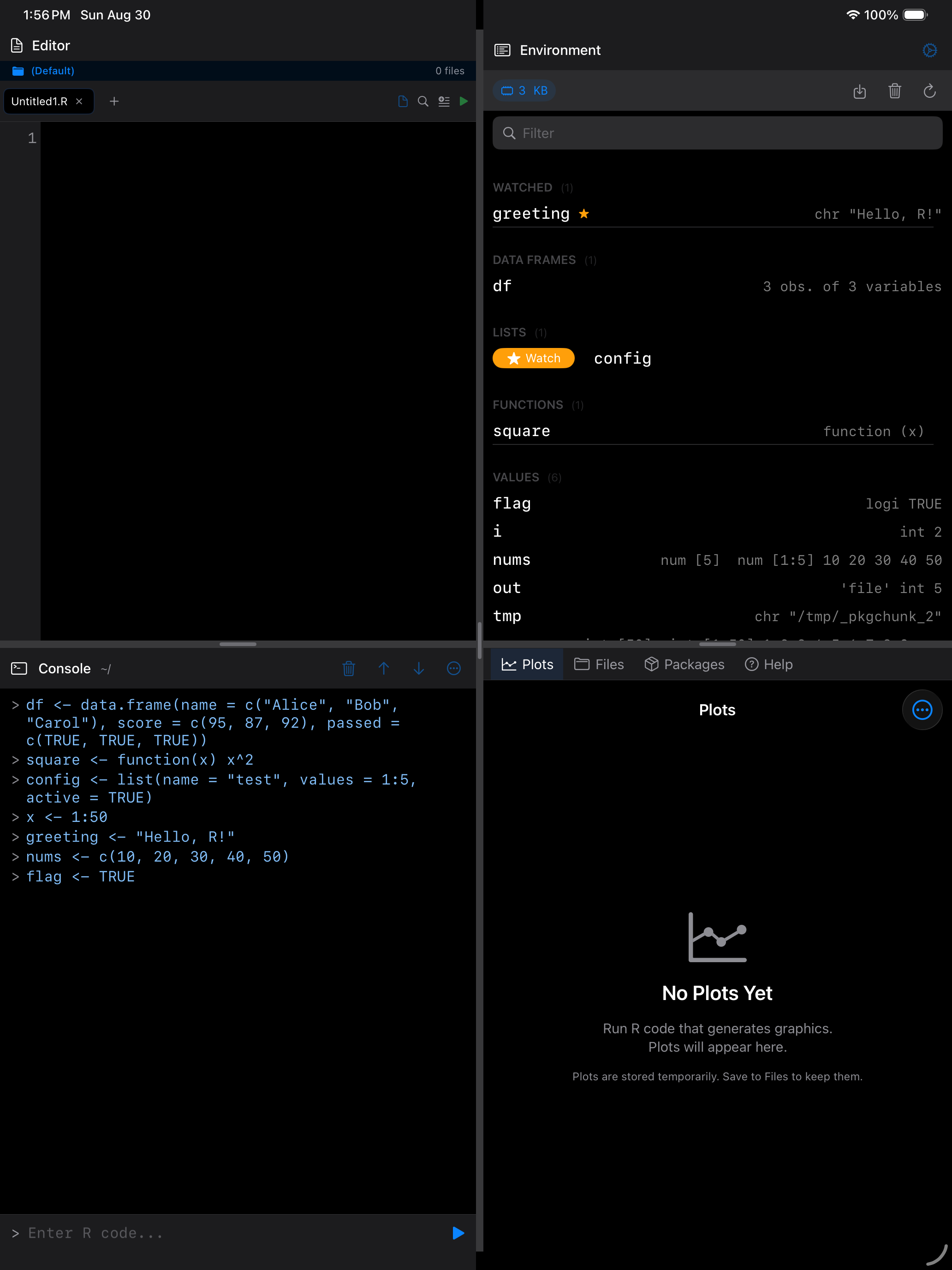
Add variables to your watch list to pin them at the top of the Environment. Useful for running totals or data frames you are building incrementally.
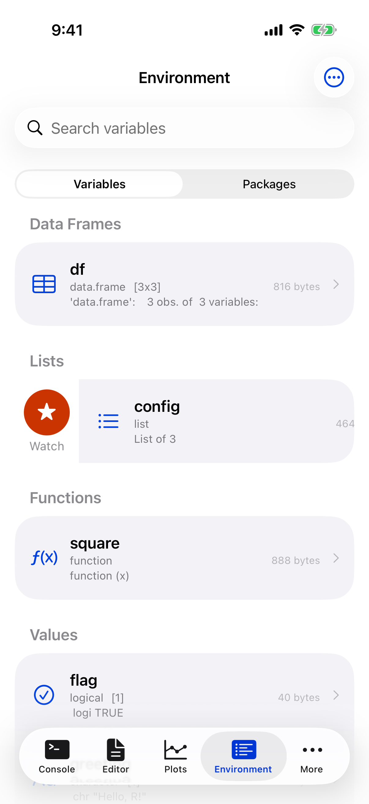
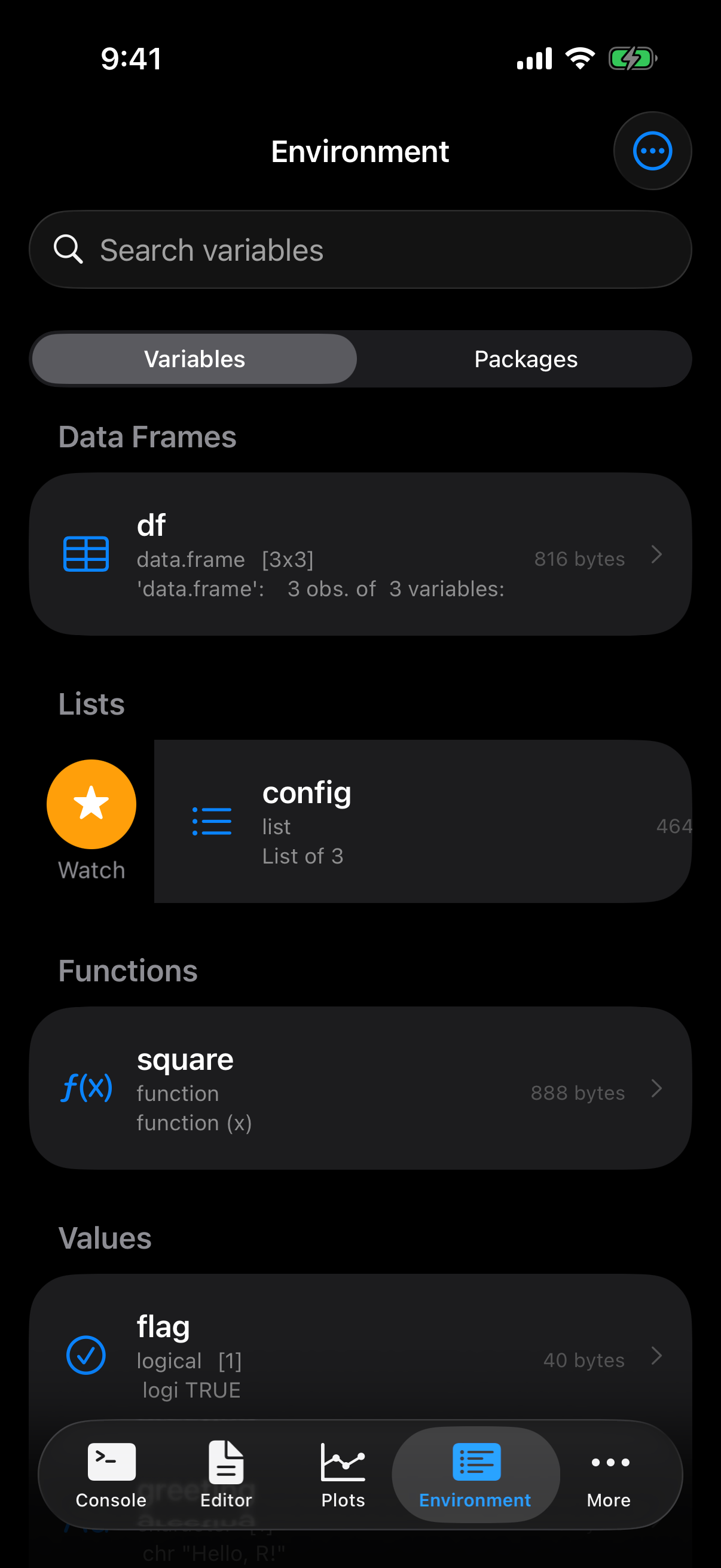
To watch a variable, swipe right on it and tap Watch. You will see a small star badge appear next to the name. To stop watching, swipe right again and tap Unwatch, or use the long-press menu.
You can clear the entire watch list at once from the menu (the ... button in the toolbar).
Searching and filtering
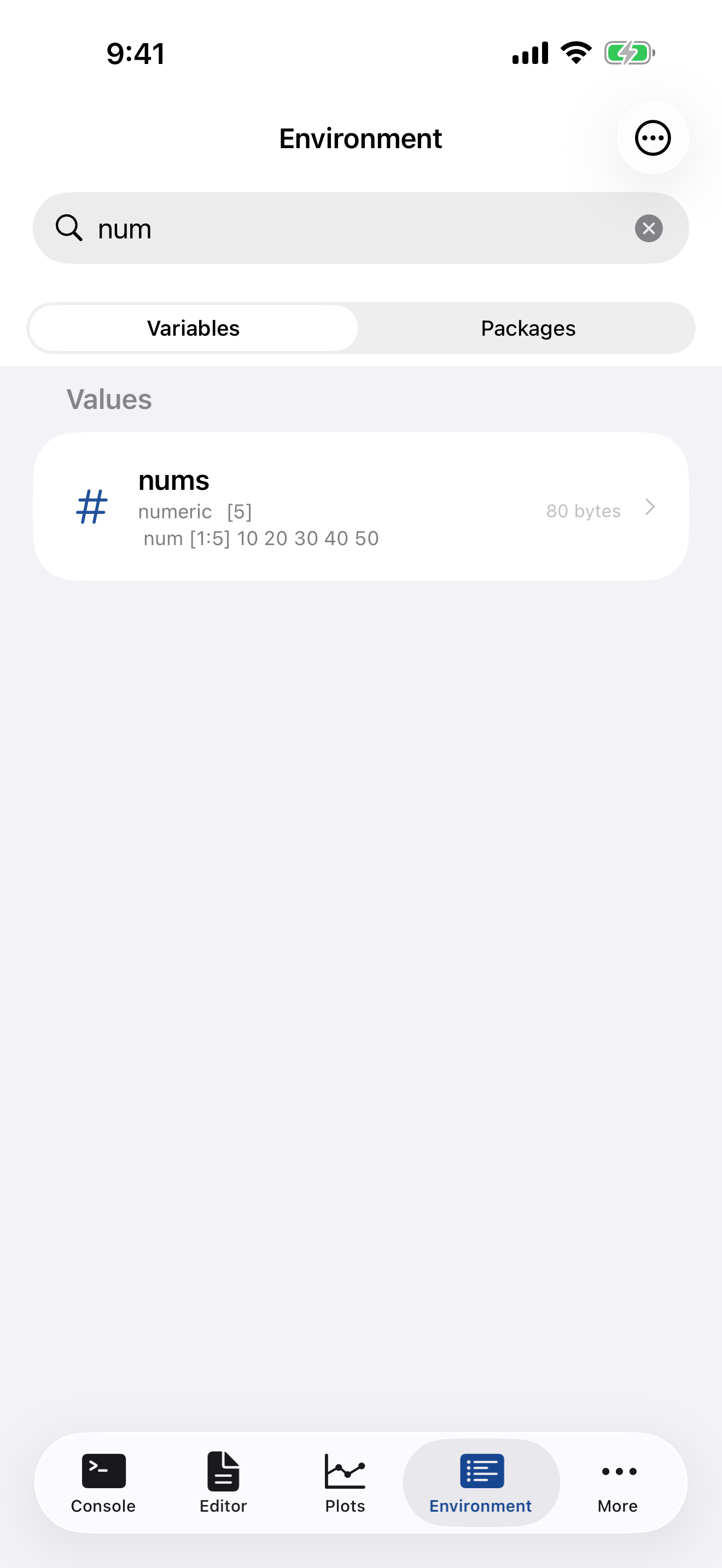
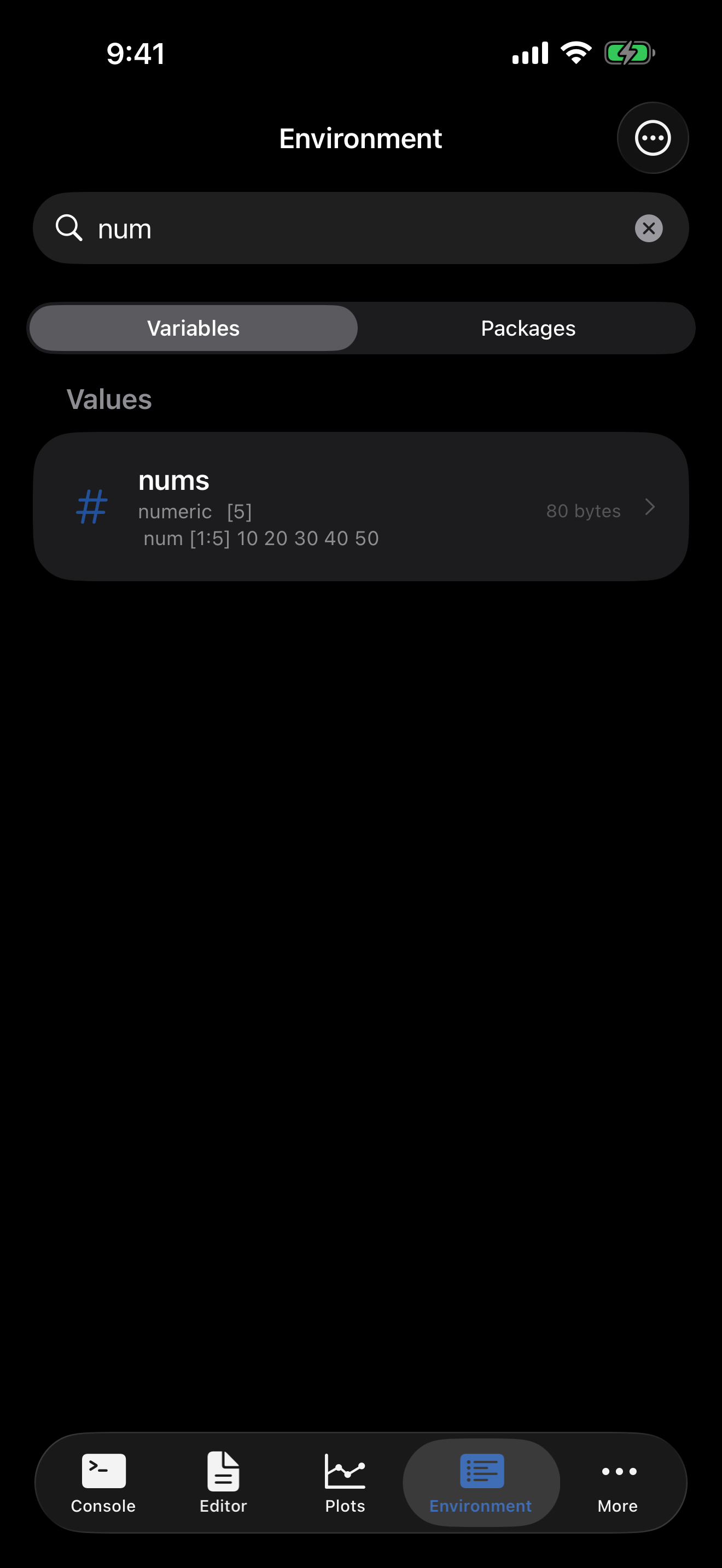
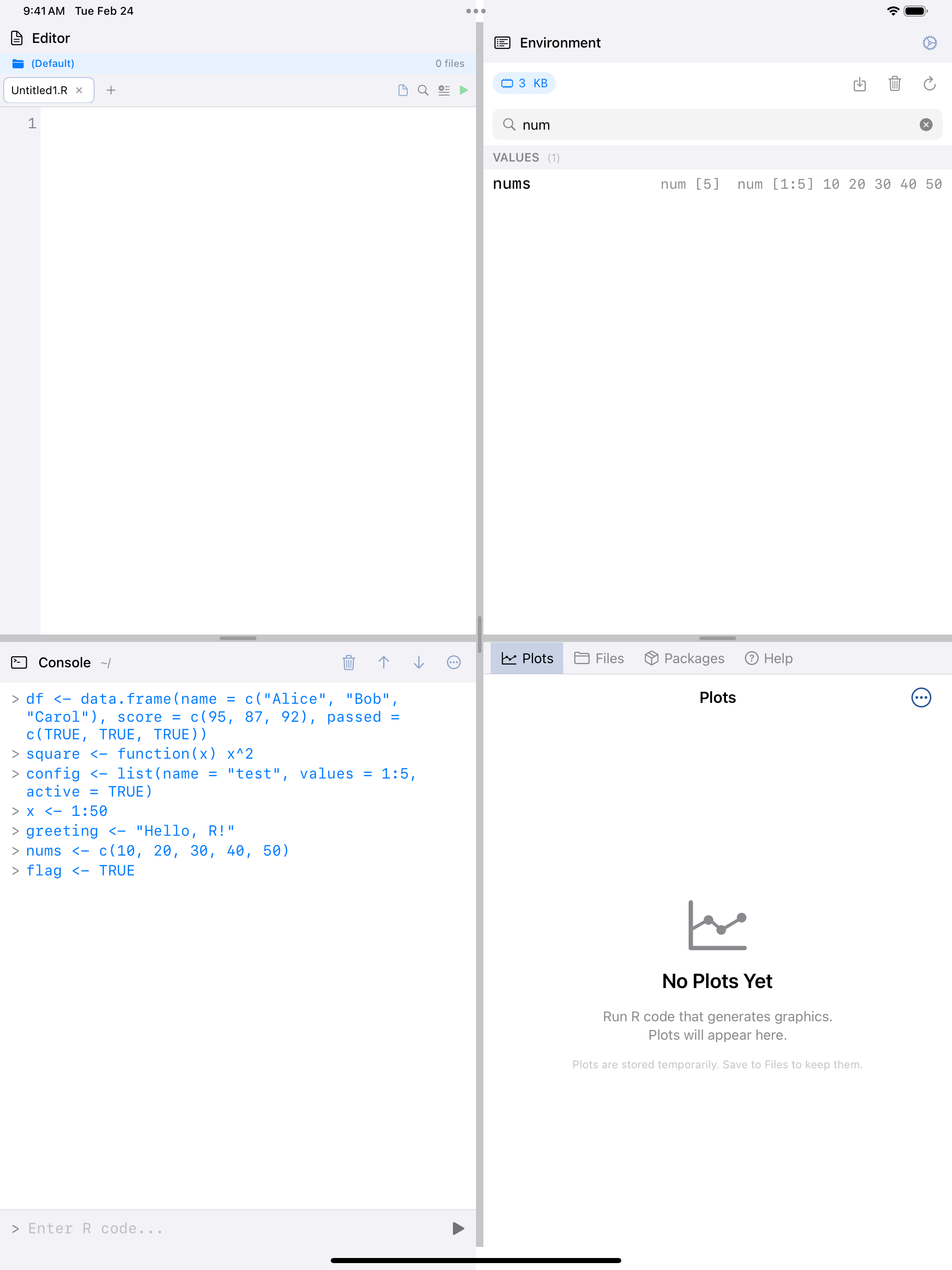
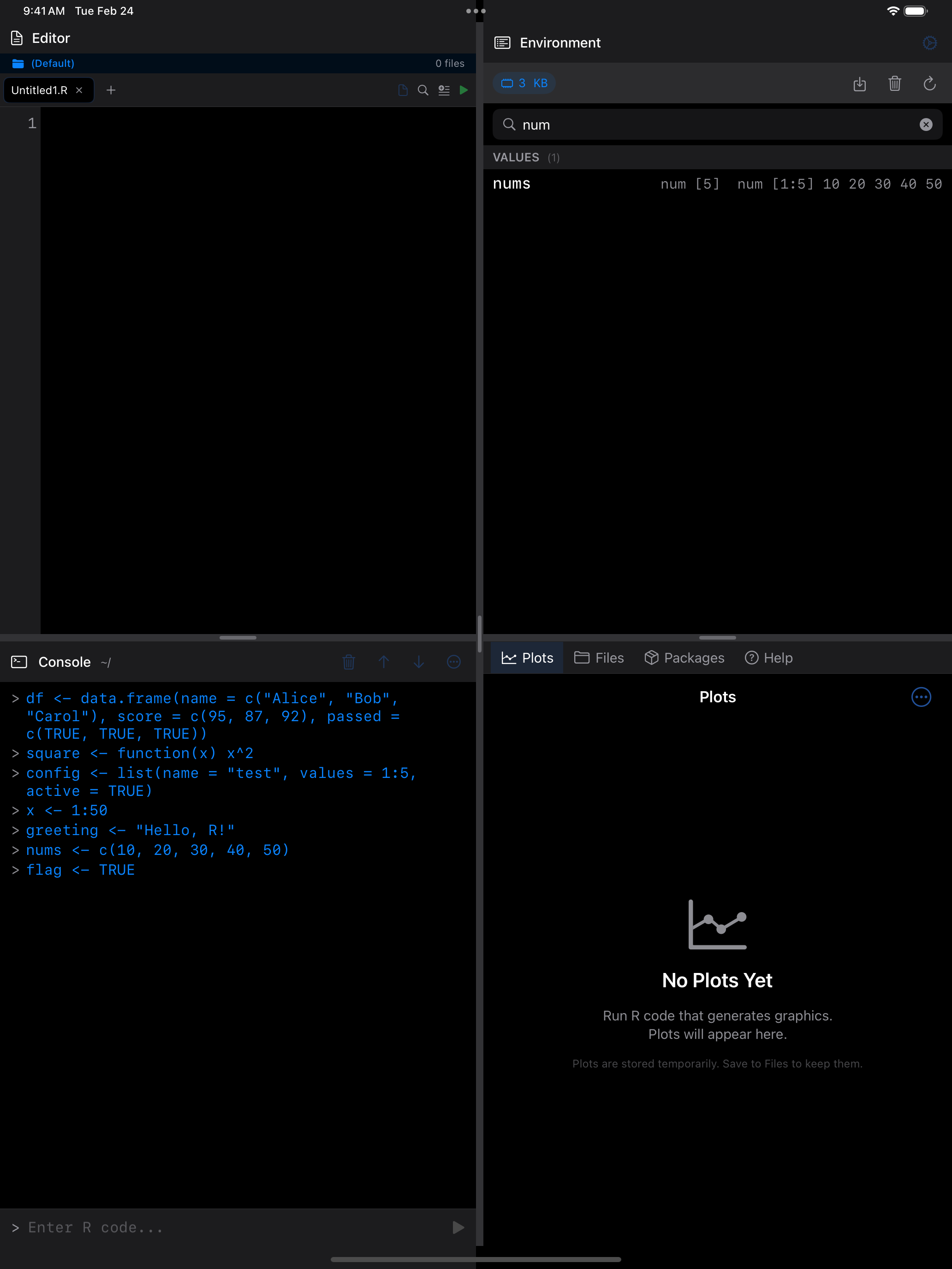
Use the search bar to filter variables by name. The list narrows as you type.
Deleting variables
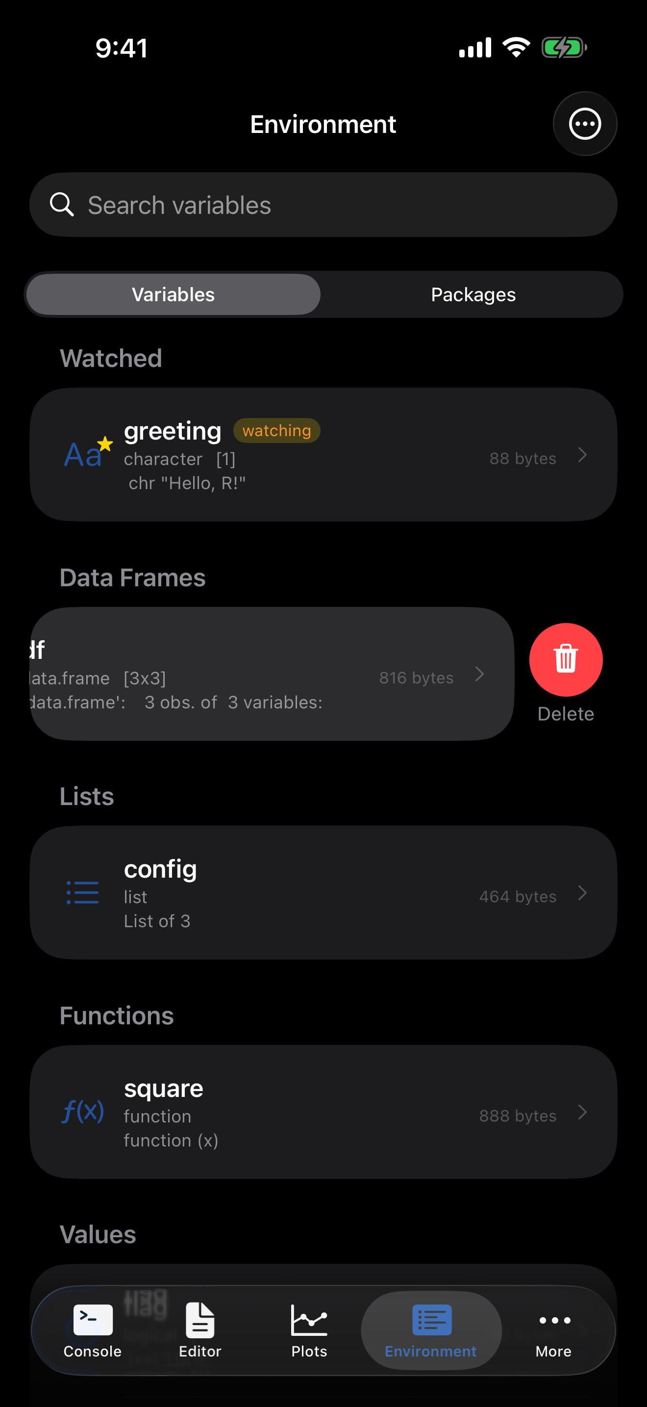
Swipe left on any variable and tap Delete to remove it (runs rm() behind the scenes). webRios asks first, and tells you if the delete fails.
To remove everything, tap the menu (...) and choose Clear Environment. This clears .GlobalEnv entirely. A confirmation prompt appears first.
The Packages tab
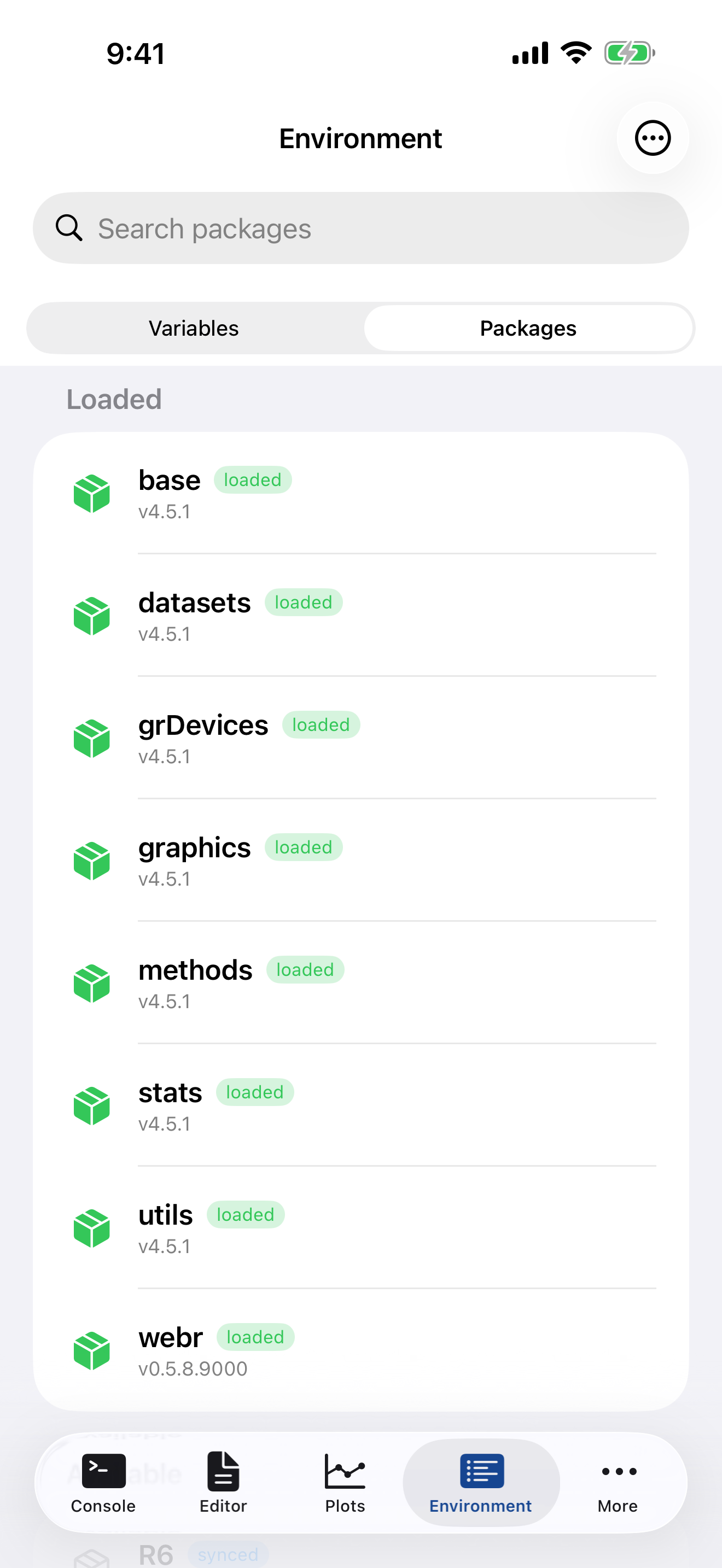
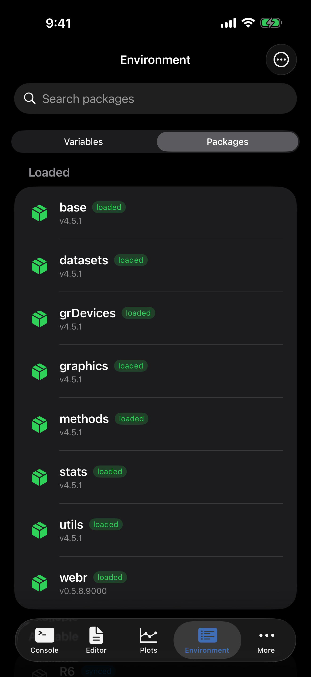
The segmented control at the top also has a Packages tab showing your installed R packages. See the Packages guide for details.
Pull down on the list to refresh manually, or tap Refresh in the menu.